Variational Autoencoders

Before delving into variational autoencoders, let's do a brief review of autoencoders.

Autoencoders

Autoencoders are a family of neural networks whose goal is to learn a simplified representation of the input data.

Their operation is based on compressing and reconstructing data. They generally consist of two networks:

1. An Encoder $g(\cdot)$ that compresses the input data $x$ into a lower-dimensional space, known as the latent space, $z = g_\phi(x)$.
2. A Decoder $f(\cdot)$ that reconstructs the data from the latent space, $x' = f_\theta(g_\phi(x))$.

The parameters of each network $(\phi, \theta)$ are optimized jointly so that the reconstructions are as similar as possible to the original data, $x \approx f_\theta(g_\phi(x))$.

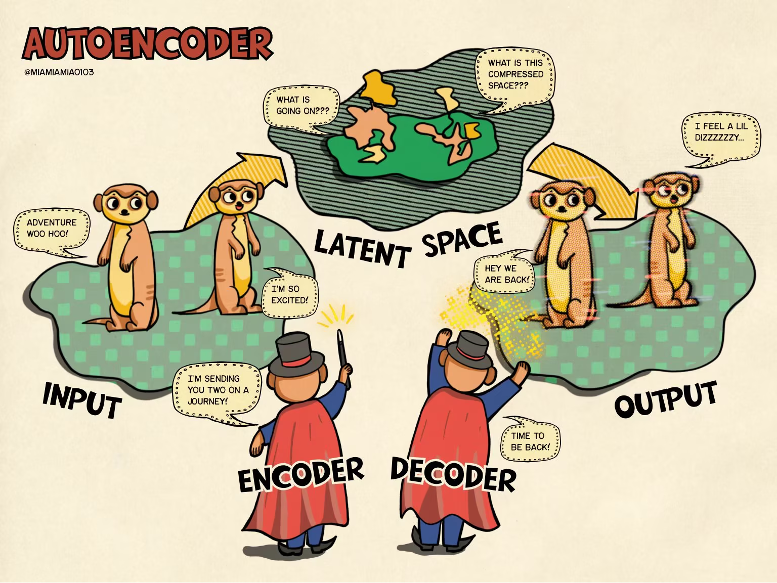
The idea originated in the 1980s and was taken up again, among other works, by Hinton and Salakhutdinov^{[hinton2006reducing]} in 2006. Today it has direct applications in tasks such as anomaly detection, manifold learning, compression, or data generation.

The loss function of a conventional autoencoder measures how well the model can reconstruct the original input once the data has been compressed into the latent space. Therefore, the goal is for the output $\hat{x}$ to be as similar as possible to the input $x$. The choice of error function depends mainly on the nature of the input data.

• Mean Squared Error (MSE)

  This is the most commonly used loss function for continuous data (for example, images or time series).

  The goal is to minimize the squared difference between the original input $x$ and the reconstructed output $\hat{x}$:

  $MSE = \frac{1}{n} \sum_{i=1}^{n} (x_i - \hat{x}_i)^2$

• Binary Cross Entropy

  This is used when the input data is normalized in the range [0, 1] and interpreted as probabilities, or when the data is binary. It is very common in autoencoders where the output layer has a sigmoid activation function.

  $BCE = -\frac{1}{n} \sum_{i=1}^{n} [x_i \log(\hat{x}_i) + (1 - x_i) \log(1 - \hat{x}_i)]$

There are many variants of autoencoders, such as Denoising Autoencoders^{[vincent2008extracting]}, Sparse Autoencoders^{[makhzani2013k]}, or Contractive Autoencoders^{[rifai2011contractive]}. From here on we will focus on Variational AutoEncoders (VAE)^{[kingma2013auto]} for their generative properties.

VAE

Conventional autoencoders map inputs to a fixed set of vectors. This means that if you sample a point in the latent space where no representation exists, the output will be unrealistic because the decoder doesn't know how to reconstruct an input from an empty region.

The novelty that VAEs introduce is that instead of mapping data to fixed vectors, they are mapped to a distribution.

Together with regularization towards a common prior, this favors a latent space that is continuous and structured. Therefore, you can choose a point $z$ that doesn't correspond exactly to the projection of any training data, pass it through the decoder, and obtain a new, coherent sample $x$. That is, generating data in the form $z \rightarrow x$.

This is precisely a generative model of latent variables.

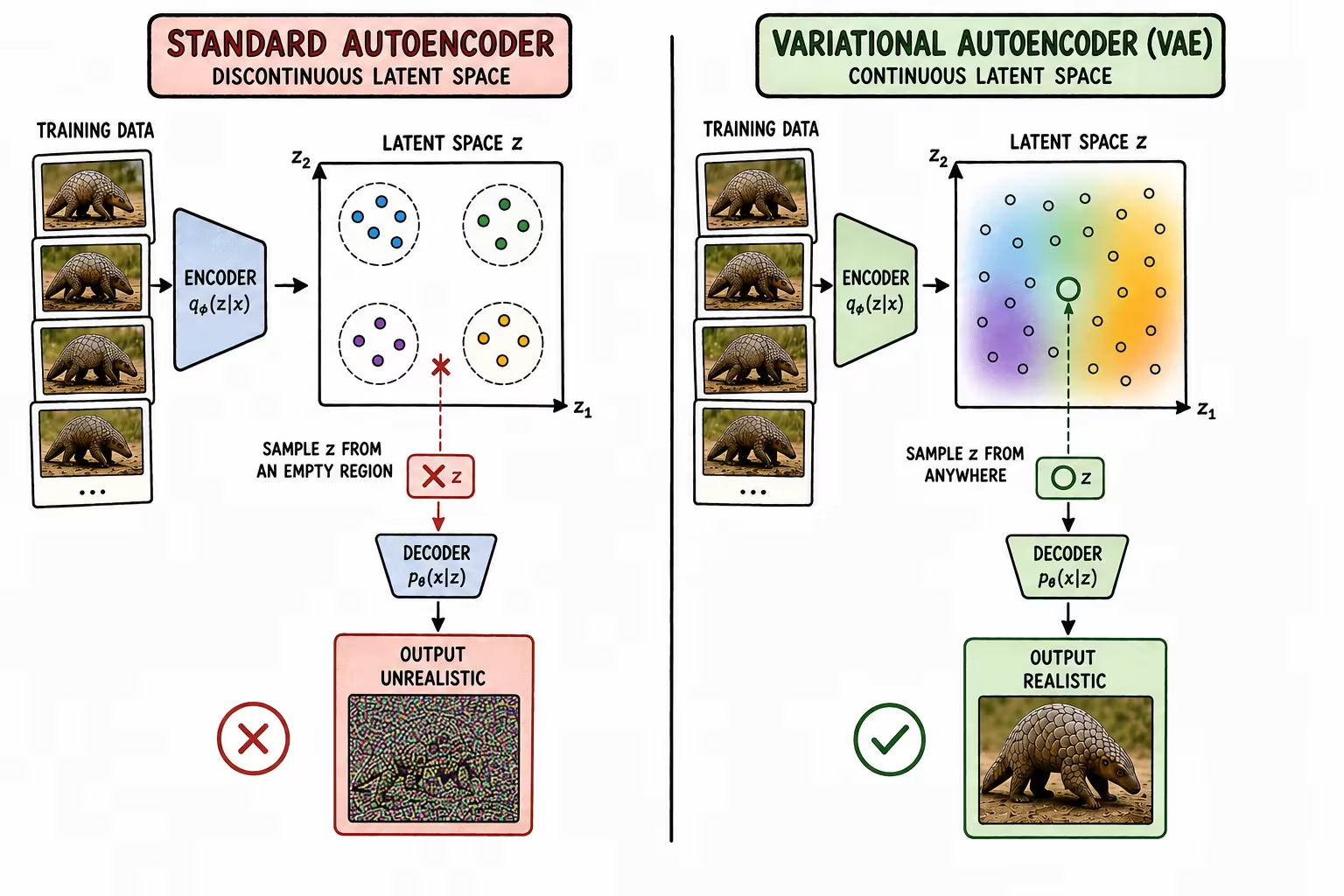
The relationship between the input data $x$ and the latent vector $z$ is given by:

• Prior: $p(z)$
• Likelihood: $p_\theta(x \mid z)$
• Posterior: $p_\theta(z \mid x)$

The distribution of the data can then be modeled as:

$p_\theta(x) = \int p_\theta(x \mid z) p(z)\, dz$

Unfortunately, $p_\theta(x)$ is not easy to compute, since it is very costly to check and sum over all possible values of $z$ (it is usually called 'intractable'). To solve this problem, VAEs resort to variational inference. Precisely, variational inference is one of the most widely used methods in Bayesian inference and is used to approximate intractable integrals. In other words, it is a technique used to approximate complex distributions.

The complex distribution we want to approximate is the posterior $p_\theta(z\mid x)$. To do this, a family of simple distributions $q_\phi(z\mid x)$ is assumed, and the approximation is posed as an optimization problem in which we search within $q_\phi$ for the distribution that best approximates the target distribution. $\phi$ denotes the parameters of the chosen family of distributions.

In this way, we introduce:

• An encoder $q_\phi(z\mid x)$ that approximates the posterior $p_\theta(z\mid x)$.
• A decoder that models the conditional probability $p_\theta(x\mid z)$.

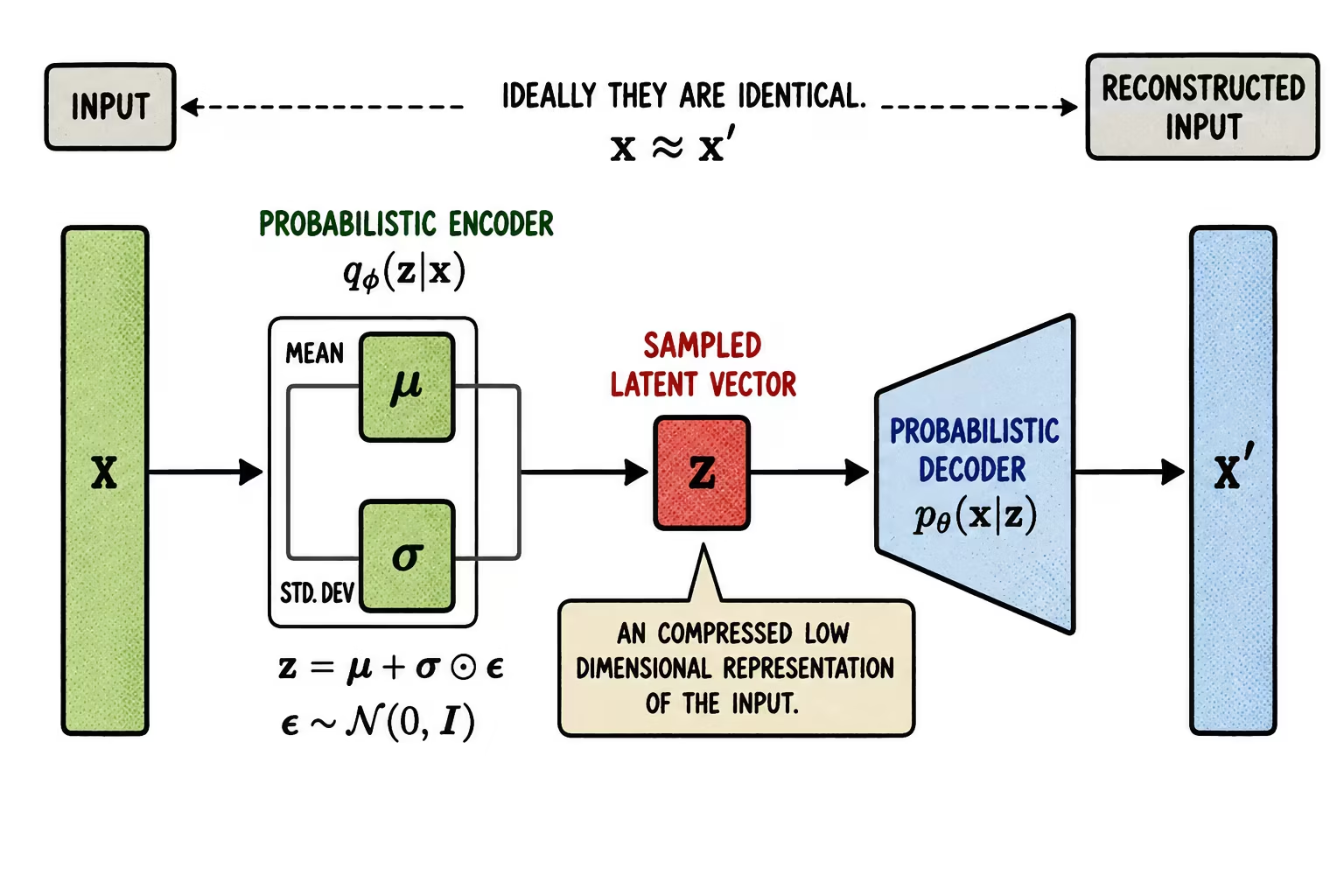
The solution to this problem is the reparametrization trick. Instead of having the network directly generate the random value $z$, the process is split into two parts:

1. The predictable part (the network): The encoder learns the mean $\mu_\phi$ and standard deviation $\sigma_\phi$ in a deterministic and differentiable way.
2. The random part ($\epsilon$): An external noise source independent of the network's weights is introduced, following a standard Gaussian distribution $\epsilon \sim \mathcal{N}(0, I)$.

Once the network and the randomness are separated, they are simply combined with:

$z = \mu_\phi(x) + \sigma_\phi(x) \odot \epsilon$

In this way, the randomness stays confined exclusively to $\epsilon$, and since it is an external variable fixed during the computation, the network doesn't need to learn how to differentiate it.

Loss function: ELBO

The distribution estimated by the encoder, $q_\phi(z\mid x)$, must approximate the true posterior $p_\theta(z\mid x)$. To quantify the distance between these two distributions, the Kullback–Leibler divergence is used, $D_{\text{KL}}(Y \| X)$, which measures how much information is lost if distribution $X$ is used to represent $Y$.

In this case we want to minimize $D_{\mathrm{KL}}(q_\phi(z\mid x)\|p_\theta(z\mid x))$ with respect to $\phi$.

Using Bayes' theorem, this can be rewritten as:

$$D_{\text{KL}}(q_\phi(z \mid x) \,\|\, p_\theta(z \mid x)) = \log p_\theta(x) - \mathbb{E}_{q_\phi(z \mid x)}[\log p_\theta(x \mid z)] + D_{\text{KL}}(q_\phi(z \mid x) \,\|\, p(z))$$

• The first term is the log-likelihood of the data, which we want to maximize.
• The second term is the expected log-likelihood of the data under the posterior approximated by the encoder.
• The third term is the KL divergence between the approximated posterior and the prior.

Combining these terms, we can define the loss function of a VAE as:

$\mathcal{L}_{\mathrm{ELBO}}(\theta, \phi; x) = \mathbb{E}_{q_\phi(z \mid x)}[\log p_\theta(x \mid z)] - D_{\mathrm{KL}}(q_\phi(z \mid x)\,\|\, p(z)),$

known as the Evidence Lower Bound (ELBO).

• The first term is the reconstruction of $x$, which tends to make the encoding-decoding scheme as efficient as possible by maximizing the log-likelihood $\log p_\theta(x \mid z)$ with sampling from $q_\phi(z \mid x)$ (encoder).
• The second term regularizes the latent variables $z$ by minimizing the KL divergence between the variational approximation (encoder) and the prior distribution of $z$. Normally, the family of simple distributions $q_\phi$ we choose is a diagonal Gaussian. Therefore, when you pass an input $x$ through the encoder, it returns the values of $\mu$ and $\sigma$ for that specific input.

The ELBO is maximized; when we talk about the loss function we minimize its negative, $-\mathcal{L}_{\mathrm{ELBO}}$.

Applications

The applications of VAEs are countless. Some examples beyond image generation are text modeling^{[yang2017improved]}, anomaly detection, remaining useful life estimation of industrial systems^{[costa2022variational]}, arrhythmia classification^{[costa2021semi]}, or molecular design^{[de2023population]}.

Posterior collapse

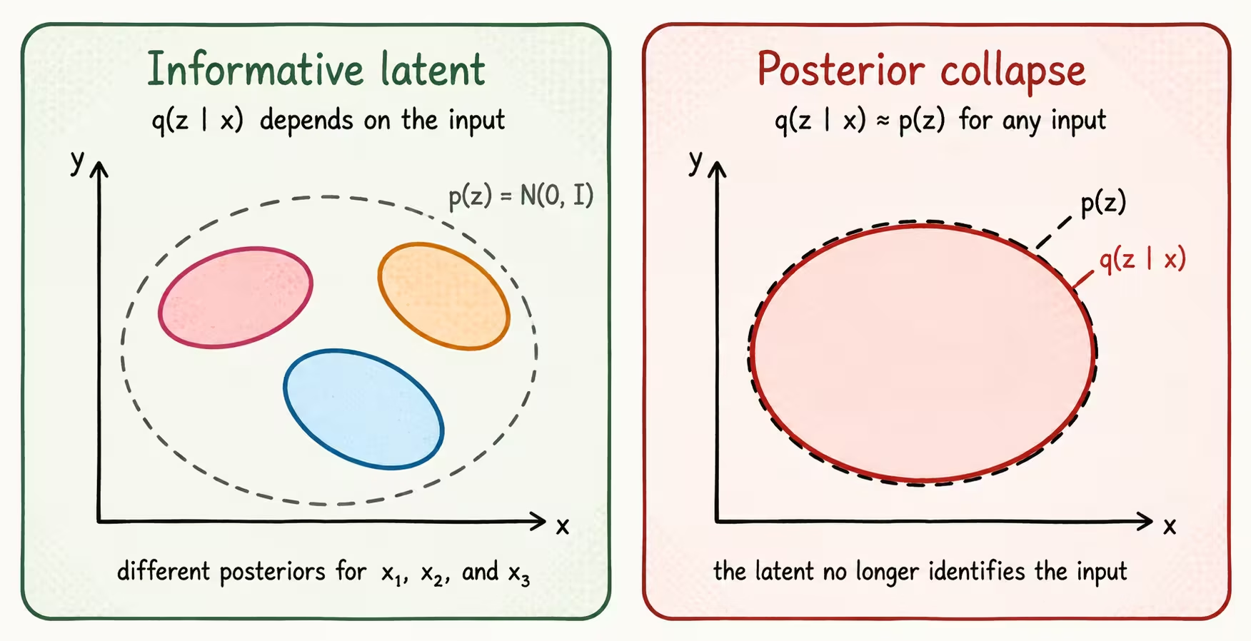
VAEs are known to be susceptible to posterior collapse. This is a problem that refers to the situation in which the posterior approximated by the encoder collapses onto the prior. That is, the encoder learns $q_\phi(z\mid x)\approx p(z)$ for any input $x$. This happens because the KL $\rightarrow$ the second term of the ELBO, is reduced to zero and the latent variables stop encoding information about the input data.

As a consequence, the decoder learns to ignore $z$ entirely and generates reconstructions based solely on global statistics of the data, nullifying the usefulness of the latent space.

Training tricks

There are several approaches to solving this problem, including:

• KL Divergence Annealing: gradually increases the weight of the KL divergence term in the loss function during training, allowing the model to first learn to reconstruct the data before imposing strong regularization on the latent space.
• Free Bits: sets a minimum threshold for the KL divergence in each dimension of the latent variable, ensuring that each one contributes at least a "minimum amount of information" and preventing them from collapsing to trivial values.
• Minimum Desired Rate: similar to Free Bits, but applies a penalty to maintain a minimum amount of information in the latent space, forcing the compression not to lose relevance.
• Limiting the decoder's capacity or adding connections from $z$: reduces the possibility of the decoder explaining the data without resorting to the latent variable.

VAE Variants

VAEs trained with a pixel-by-pixel reconstruction loss tend to produce blurry images. Why does this happen?

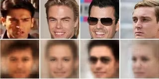
Typically, metrics such as RMSE or BCE are used to quantify the quality of the reconstructions, as we mentioned earlier. Therefore, the network's goal is to minimize these metrics.

The problem arises when, for the same latent representation, several plausible reconstructions exist. In that case, to minimize a pixel-by-pixel loss, the network can make a kind of cheat: predicting intermediate values between those alternatives. In an image, that conditional average between possibilities tends to produce blurry edges and details.

β-VAE

One way to control the balance between reconstruction quality and latent space regularization is to introduce a hyperparameter $\beta$ that adjusts the weight of the KL term:

$\mathcal{L}(\theta, \phi; x) = \mathbb{E}_{q_\phi(z \mid x)}[\log p_\theta(x \mid z)] - \beta\, D_{\text{KL}}(q_\phi(z \mid x) \,\|\, p(z))$

This is what the β-VAE^{[higgins2017beta]} consists of.

If $\beta = 1$ is set, the objective function is the same one used in standard VAEs; if it is set to 0, the KL regularization disappears and the objective is reduced to the reconstruction term, bringing the behavior closer to that of a conventional autoencoder.

If $\beta < 1$ is used, more bits are stored about each input (that is, more importance is given to the data) and, therefore, images can be reconstructed in a less blurry way. On the other hand, an advantage of using $\beta > 1$ is that it encourages learning a "disentangled" latent representation. Intuitively, this means that each latent dimension represents a different factor/feature of the input data. For example, a model trained on photos of human faces might capture smoothness, skin color, hair color or length, emotion, whether glasses are worn, and many other relatively independent factors in separate dimensions.

In summary: designing a VAE is almost always a balancing act between "I want the reconstruction to look good" and "I want the latent space to make sense."

InfoVAE

To solve the problem of placing too much emphasis on the second term (regularization), causing latent representations that don't capture the structure of the data well and generated samples that lack diversity, InfoVAE^{[zhao2017infovae]} modifies the loss function by adding a mutual information maximization term between the latent variables $z$ and the observed data $x$. The InfoVAE loss function can be written as:

$$\mathcal{L}_{\text{InfoVAE}} = \mathbb{E}_{p_{\mathrm{data}}(x)} \left[ \mathbb{E}_{q_\phi(z\mid x)} [\log p_\theta(x\mid z)] - (1-\alpha) D_{\mathrm{KL}}\!\left(q_\phi(z\mid x)\,\|\,p(z)\right) \right] - (\alpha+\lambda-1) D_{\mathrm{KL}}\!\left(q_\phi(z)\,\|\,p(z)\right)$$

Where the first term is the reconstruction error, the second is the KL divergence between the approximated posterior distribution and the prior, and the third is the KL divergence between the marginal distribution of the latent variables and the prior distribution. The distribution $q_\phi(z)=\int q_\phi(z\mid x)\,p_{\mathrm{data}}(x)\,dx$ is known as the aggregated posterior and describes how the encodings of the entire dataset are distributed in the latent space.

$\alpha$ and $\lambda$ are hyperparameters that control the relative importance of each term. In this way, the objective favors $z$ retaining information about $x$ while still approximating the aggregated posterior to the prior.

Multimodal VAEs

Multimodal VAEs^{[wu2018multimodal]}, ^{[shi2019variational]} are an extension of the standard VAE model to handle and learn joint representations of data coming from different modalities. These modalities can include text, images, audio, video, etc. The main idea is to capture the dependencies and correlations between different types of data, learning a shared latent representation that can be used for tasks such as data generation or imputation.

Several approaches have been proposed so far for multimodal VAE learning. This review gathers some of the most influential works.

Hierarchical VAEs

One limitation of standard VAEs is that they usually use a simple prior, such as a standard Gaussian. One way to increase their flexibility is to introduce a hierarchy of latent variables. By making both the inference model (encoder) and the generative model (decoder) hierarchical, more complex distributions can be represented.

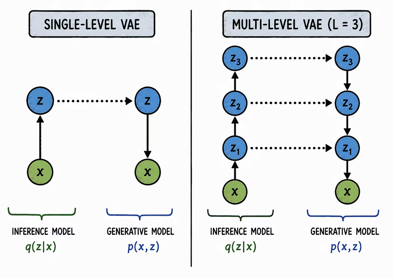
The distribution we want to model then is:

$p(x) = \int p(x \mid z_1)\, p(z_1 \mid z_2) \cdots p(z_k)\, dz_{1:k},$

Therefore, the ELBO would be expressed as follows:

$\mathcal{L}_{\mathrm{ELBO}} = \mathbb{E}_{q(z_{1:k}\mid x)}[\log p(x \mid z_1)] - D_{\mathrm{KL}}\!\left(q(z_{1:k}\mid x)\,\|\,p(z_{1:k})\right)$

Many hierarchical models have been published, among which VD-VAE (Very Deep VAE)^{[child2020very]} stands out for image generation, and Bit-Swap^{[kingma2019bit]} for data compression.

The VD-VAE architecture is a convolutional VAE. For each group of latent variables, the prior and posterior are diagonal Gaussians. In the decoder, it uses nearest-neighbor resampling instead of transposed convolutions and adds several design decisions to stabilize training. Together, this makes it possible to train a deep hierarchy using the original ELBO, without modifying the objective function.

Extra: Compression

In Bit-swap^{[kingma2019bit]}, a hierarchical VAE is presented, demonstrating that the bits-back compression scheme (BB-ANS) can be used with latent variable models. That is, this type of generative model can be used as efficient compression schemes. Let's take a look, but first: a bit of information theory.

Kolmogorov complexity

In information theory, the Kolmogorov complexity of an object $x$, denoted $K(x)$, refers to the length of the shortest possible description of that object on a 'universal computer'. It represents the inherent complexity of a piece of information $x$ as a function of the length of the most concise binary program capable of generating it.

$\rightarrow$ A shorter binary program implies a higher level of regularity or predictability in the data.

$\rightarrow$ A longer binary program suggests a more complex, less compressible structure.

Similarly, the Kolmogorov complexity of $x$ given $y$, $K(x|y)$, corresponds to the length of the binary program that, receiving $y$ as input, produces $x$. Based on this idea, Bennett et al. ^{[bennett1998information]} derived the information distance metric, $E(x,y)$:

$$E(x,y)=\max\{K(x\mid y),K(y\mid x)\}=K(x,y)-\min\{K(x),K(y)\}+O(\log K)$$

This metric essentially evaluates the existence of a simple program capable of transforming one object into another and, therefore, provides a measure of the relationship or amount of information shared between them. The simpler the conversion program, the more similar the objects are considered to be. However, Kolmogorov complexity is not theoretically computable but can only be approximated.

Compression

Compression techniques approximate Kolmogorov complexity, since they offer a practical means of representing data more concisely without losing essential information. The main goal of a lossless compressor is to minimize the number of bits needed to represent the data, subsequently allowing its exact decompression.

Compression methods achieve this goal by identifying and exploiting redundancies or patterns present in the data. To achieve the shortest possible compression length, symbols with higher probability receive shorter codes. According to Shannon's Source Coding Theorem ^{[shannon1948mathematical]}, the length of the encoded bits is directly related to the entropy of the information source:

What compression algorithms seek is to effectively model the "real" distribution of the data $p(x)$:

• A common strategy consists of dictionary-based methods, where patterns or sequences of data are identified and replaced with shorter codes. Among these are the Lempel-Ziv algorithms, which dynamically build a dictionary during compression ^{[kosaraju2000compression]}.

• Context-based models, such as adaptive arithmetic coding, adjust the encoding probabilities based on the context of previously encoded symbols ^{[moffat1998arithmetic]}.

• Entropy coding methods, such as Huffman coding, assign shorter prefix codes to the most probable symbols ^{[moffat2019huffman]}.

Recent advances have incorporated Machine Learning techniques into compression algorithms. What models can we use to approximate the real distribution of the data?

$\rightarrow$ Exactly, VAEs!!

Generative models as compressors

In a typical compression pipeline, data is represented as a sequence of symbols $X = x_1, x_2, ..., x_n$ and encoded into a set of bits $C$. Afterwards, the inverse process is applied to recover the original data.

• Compression: $E(X) \rightarrow C$

• Decompression: $D(C) \rightarrow X'$

Lossless compression methods seek to minimize the number of bits without sacrificing information. For a symbol with probability $p(x)$, the ideal length is $-\log_2 p(x)$ bits.

The better the compression, the better the approximation of $p(x)$. In a probabilistic context, $p(x)$ can be expressed as the probability of observing the data under a given model:

$$p(x) = \int p(x|\theta) p(\theta) d\theta$$

where $p(x|\theta)$ is the probability of observing the data given a specific set of parameters, $p(\theta)$ is the prior distribution, and $\theta$ represents the model's parameters.

In the context of generative modeling, this expression is usually formulated in terms of the latent variable $z$:

$$p(x) = \int p(x|z) p(z) dz$$

Sounds familiar, right?

Using this notation, the process of sending information in a compression scheme ($E(X)\rightarrow C$) proceeds as follows:

1. The latent variable $z$ is encoded using $p(z)$.
2. The sample $x$ is encoded using $p(x|z)$.
3. Both $z$ and $x$ are transmitted.

On the other hand, receiving the information ($D(C)\rightarrow X'$) follows these steps:

1. $z$ is decoded using $p(z)$.
2. $x$ is decoded using $p(x|z)$.

The number of bits involved initially corresponds to $-\log_2 p(z)-\log_2 p(x\mid z)$. The bits-back method allows recovering approximately $-\log_2 q(z\mid x)$ bits used to select $z$^{[frey1997efficient]}. This idea connects variational inference with probabilistic compression.

The compression process described above can be interpreted according to the BB-ANS scheme ^{[townsend2019practical]}. Some extra bits are used to generate a sample $z$ via the encoder $q(z|x)$; afterwards, $z$ is used to encode $x$ through $p(x|z)$, while the variable $z$ itself is encoded using the prior distribution $p(z)$. The reverse process allows recovering $z$ via $p(z)$, reconstructing $x$ via $p(x|z)$, and recovering the initial extra bits using $q(z|x)$.

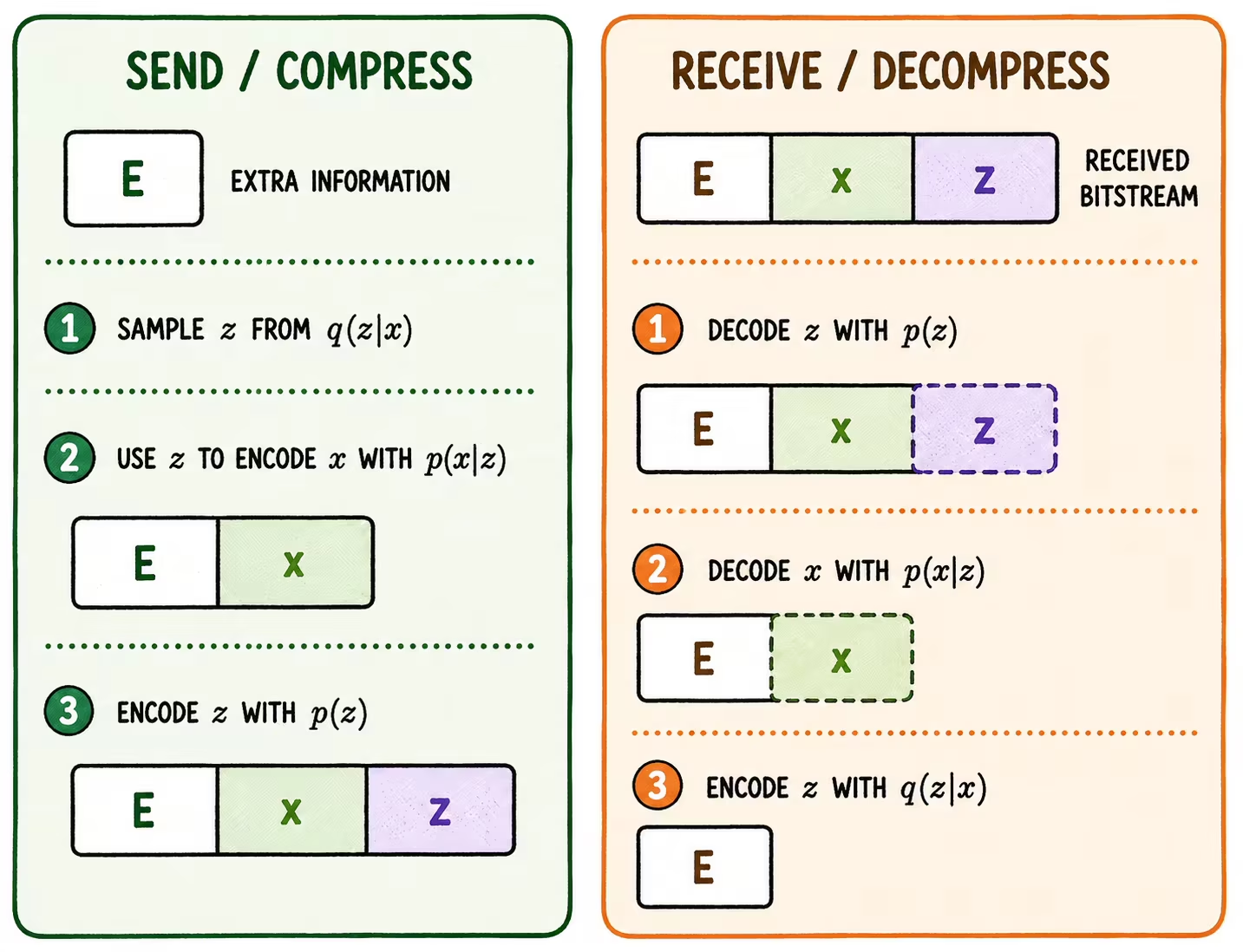
The final length of the bit stream for a single data point is given by:

$$N=n_{\mathrm{extra}}+\log_2 q(z\mid x)-\log_2 p(x\mid z)-\log_2 p(z)$$

Notice that the costs $-\log_2 p(z)$ and $-\log_2 p(x\mid z)$ are transmitted, but the bits-back mechanism allows recovering approximately the $-\log_2 q(z\mid x)$ extra bits used to select $z$. What matters here is that $N-n_{\mathrm{extra}}$ coincides with the negative ELBO (negative Evidence Lower Bound, nELBO), expressed in bits:

$$\mathbb E_{q(z\mid x)}[N-n_{\mathrm{extra}}] = \mathbb E_{q(z\mid x)}\left[\log_2\frac{q(z\mid x)}{p(x,z)}\right] =-\mathcal L_{\mathrm{ELBO}}/\log 2$$

Dividing by $\log 2$ converts nats into bits. This cost corresponds to the loss function we minimize in a VAE.

$$\mathcal L_{\mathrm{ELBO}} = \mathbb E_{q(z\mid x)} \left[\log\frac{p(x,z)}{q(z\mid x)}\right] = \mathbb E_{q(z\mid x)}\left[\log\frac{p(x\mid z)p(z)}{q(z\mid x)}\right] = \mathbb E_{q(z\mid x)}\left[\log p(x\mid z)\right] + \mathbb E_{q(z\mid x)}\left[\log\frac{p(z)}{q(z\mid x)}\right] = \mathbb E_{q(z\mid x)}\left[\log p(x\mid z)\right]-D_{\mathrm{KL}}\left(q(z\mid x)\|p(z)\right)$$

• The first term corresponds to the reconstruction of $x$ and favors an efficient encoding and decoding scheme by maximizing $\log p(x\mid z)$ with samples from $q(z\mid x)$.

• The second term is the regularization of the latent space by minimizing the KL divergence between the variational approximation and the prior distribution $z$.

As a result, minimizing the negative ELBO maximizes a lower bound of $\log p(x)$ and brings $q(z\mid x)$ closer to the model's posterior $p(z\mid x)$.

This equivalence demonstrates that a properly optimized latent variable model, such as a VAE, is directly applicable to compression tasks, since it minimizes the achievable code length in the context of bits-back coding.

Jiang et al., in NPC (Non-Parametric learning by Compression)^{[jiang2022few]}, proposed a method based on this premise for image classification, outperforming supervised and semi-supervised methods.

Similarly, in Few-shot generative compression approach for system health monitoring ^{[costa2025few]} I proposed a method based on compression and VAEs to diagnose cases where monitoring data is abundant, but there are very few labeled instances.