Diffusion models

Introduction

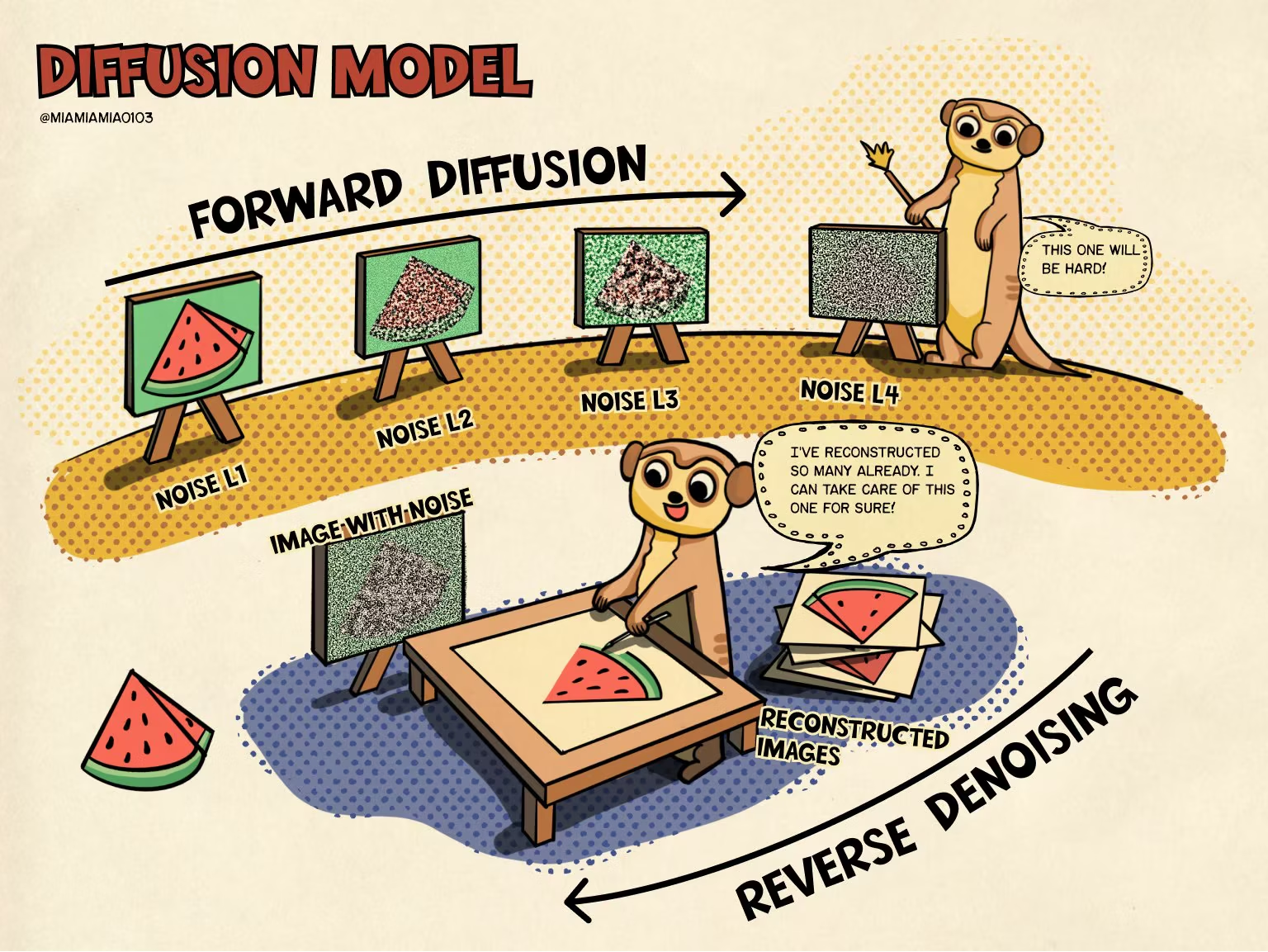
Diffusion models draw inspiration from non-equilibrium thermodynamics. They add noise to the data and then learn a reverse process that generates samples from noise.

Specifically, a diffusion process is applied to gradually convert the observed data $x_0$ into a noisy version $x_T$ by repeatedly passing the data through a stochastic encoder $q(x_t \mid x_{t-1})$. After enough steps, we end up with $x_T \approx \mathcal{N}(0, I)$, or any other convenient reference distribution. Then, a reverse process is learned by passing the noise through $T$ steps of a decoder $p(x_{t-1} \mid x_t)$ until $x_0$ is generated again.

These models are similar to hierarchical VAEs, in the sense that they have an encoder and a decoder and follow a sequence of steps or hierarchies, and also to normalizing flows, since they apply a sequence of transformations to the data.

Remember the image from the beginning of the course? It should make much more sense now.

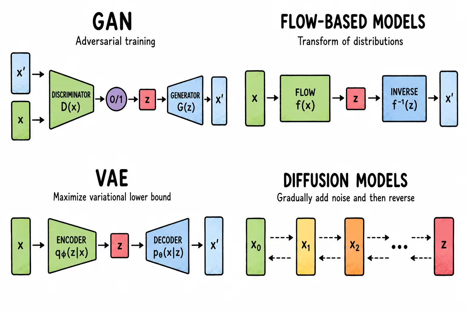
In diffusion models, the forward process in which we add noise is not learned but instead follows a fixed procedure, and the latent variable has the same dimensionality as the original data. On the other hand, the decoder is shared across all steps.

Several diffusion-based generative models have been proposed, including diffusion probabilistic models^{[sohl2015deep]}, noise-conditioned score network^{[song2019generative]}, denoising diffusion probabilistic models^{[ho2020denoising]}, and variational diffusion models^{[kingma2021variational]}.

Encoder (forward diffusion)

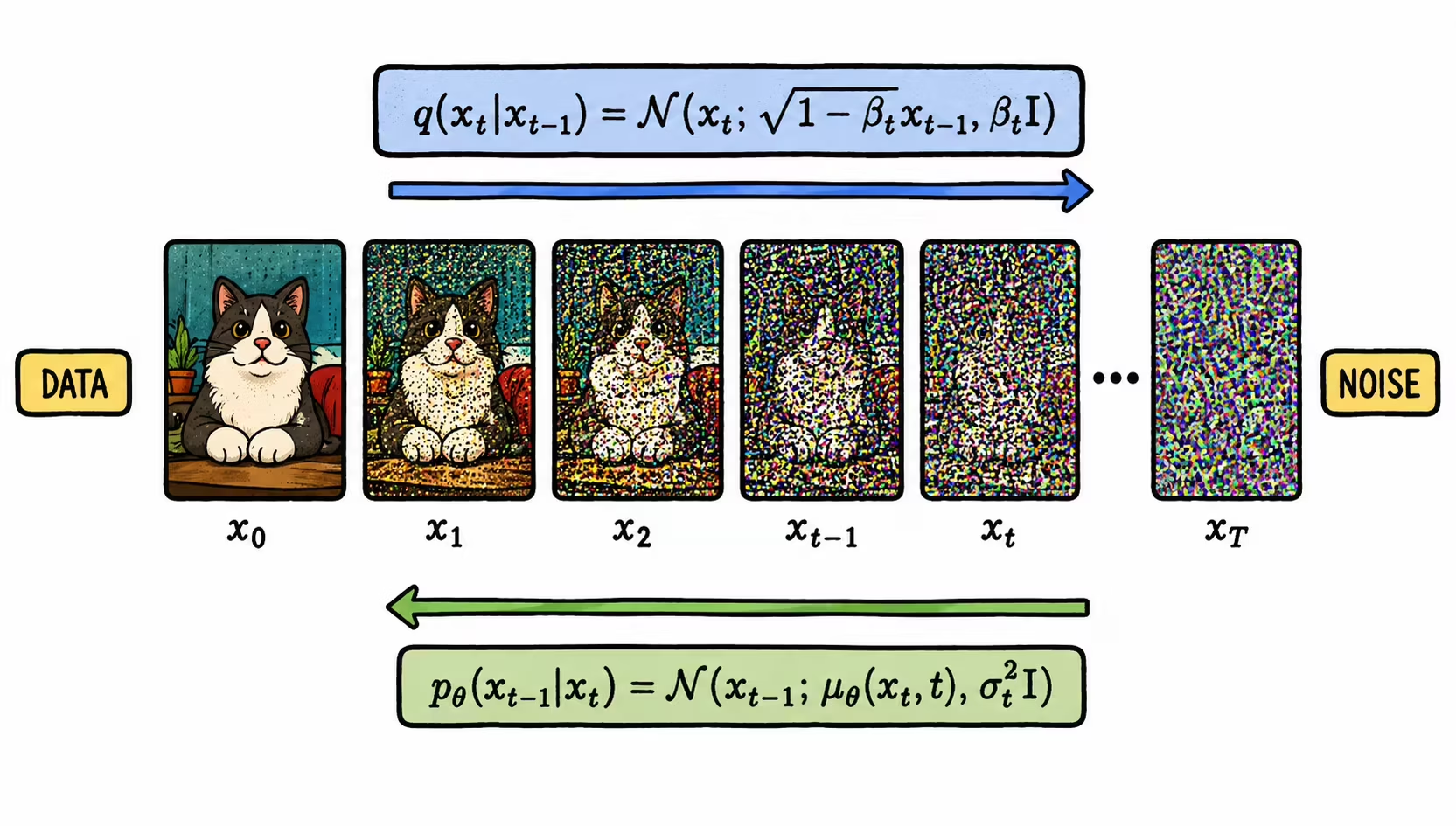
Forward diffusion is the easy part because it doesn't involve training any model. It is a fixed procedure in which we decide how to add noise.

The process is usually defined as a simple linear Gaussian model:

$$q(\mathbf{x}_t \mid \mathbf{x}_{t-1}) = \mathcal{N}\!\left( \mathbf{x}_t \,\middle|\, \sqrt{1 - \beta_t}\, \mathbf{x}_{t-1},\, \beta_t \mathbf{I} \right),$$

where the values of $\beta_t \in (0, 1)$ are chosen according to a noise scheduler.

Intuitively, $\beta_t$ controls how much noise we add at each step $t$:

• if $\beta_t$ is small, the image changes very little
• if $\beta_t$ is large, we add a lot of noise at once

The noise scheduler decides how that amount of noise grows throughout the process. Adding a lot of noise from the start is not the same as adding it slowly and accelerating toward the end.

The joint distribution over the latent states is:

$$q(\mathbf{x}_{1:T} \mid \mathbf{x}_0) = \prod_{t=1}^{T} q(\mathbf{x}_t \mid \mathbf{x}_{t-1})$$

The distribution $q(\mathbf{x}_t \mid \mathbf{x}_0)$ is known as the diffusion kernel. Applying this to the input data distribution and then computing the resulting unconditional marginals is equivalent to Gaussian convolution:

$$q(\mathbf{x}_t) = \int q_0(\mathbf{x}_0)\, q(\mathbf{x}_t \mid \mathbf{x}_0)\, d\mathbf{x}_0$$

As $t$ increases, the signal-to-noise ratio decreases and the marginals approach a simple distribution. In images, this process first removes high-frequency content (i.e., low-level details, such as texture), and then low-frequency content (high-level or "semantic" information, such as shape).

Decoder (reverse diffusion)

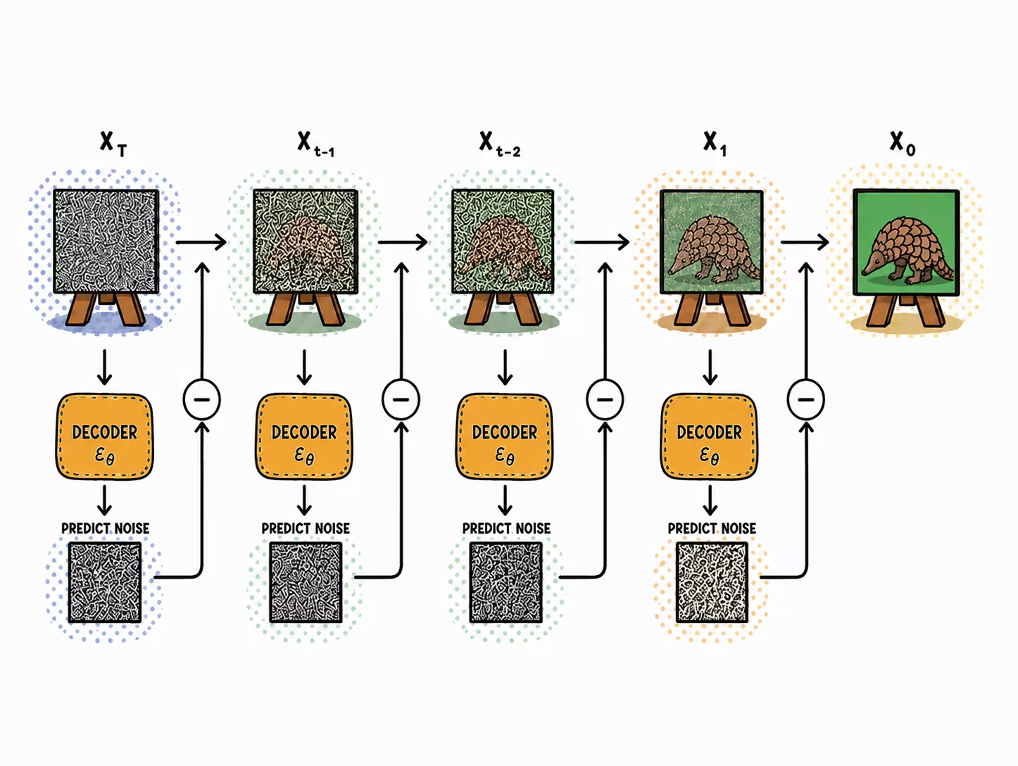
The ultimate goal of a diffusion model is for the reverse process (decoder) to learn the original data distribution, $p(x_0)$.

By adding noise in $T$ steps, a sequence of intermediate distributions $q(x_t \mid x_0)$ is created, where $x_t$ is the original data $x_0$ with an increasing amount of noise.

Generating a full image from scratch is hard, so the problem is reformulated to consist 'only' of removing a bit of noise from a given image. By doing it in several steps, we turn a complicated task into many simple ones.

In other words, to generate a new sample we don't know $x_0$, so we train a model to approximate the reverse distribution:

$$p_\theta(\mathbf{x}_{t-1} \mid \mathbf{x}_t) = \mathcal{N}\!\left( \mathbf{x}_{t-1} \,\middle|\, \mu_\theta(\mathbf{x}_t, t),\, \Sigma_\theta(\mathbf{x}_t, t) \right)$$

The corresponding joint distribution over all generated variables is given by:

$$p_\theta(x_{0:T}) = p(x_T) \prod_{t=1}^{T} p_\theta(x_{t-1} \mid x_t), \quad \text{where } p(x_T) = \mathcal{N}(0, I)$$

To generate data from the model, a point $x_T \sim \mathcal{N}(0, I)$ is sampled and then the Markov chain is run backward, sampling $x_t \sim p_\theta(x_t \mid x_{t+1})$ until a sample is obtained in the original data space, $x_0$.

Training

We have already defined the two processes that make up a diffusion model: the forward process adds noise through known transitions, and the reverse process progressively tries to recover the data. What's left is to learn the parameters $\theta$ of each reverse transition $p_\theta(x_{t-1}\mid x_t)$.

During training we start from a clean sample $x_0$, so we can generate any noisy state $x_t$ and compute what the step toward $x_{t-1}$ should look like. The goal is to get the learned transition to approximate that reverse process. This idea is formulated probabilistically through the ELBO and ends up producing a simple noise-prediction loss.

The ELBO as a starting point

We want to maximize the log-likelihood of the data, $\log p_\theta(x_0)$, but computing it requires integrating over all latent states $x_{1:T}$. As in a VAE, we use the forward process $q(x_{1:T}\mid x_0)$ as the variational distribution and minimize the negative ELBO:

$$\mathcal{L}_{\mathrm{VLB}} = \mathbb{E}_{q} \left[ -\log \frac{p_\theta(x_{0:T})}{q(x_{1:T}\mid x_0)} \right]$$

*VLB stands for "Variational Lower Bound".

This expression can be decomposed into a sum of local problems:

$$\mathcal{L}_{\mathrm{VLB}} = \underbrace{D_{\mathrm{KL}}\!\left(q(x_T\mid x_0)\,\|\,p(x_T)\right)}_{\mathcal{L}_T} + \sum_{t=2}^{T} \underbrace{D_{\mathrm{KL}}\!\left(q(x_{t-1}\mid x_t,x_0)\,\|\,p_\theta(x_{t-1}\mid x_t)\right)}_{\mathcal{L}_{t-1}} + \underbrace{-\log p_\theta(x_0\mid x_1)}_{\mathcal{L}_0}$$

• $\mathcal{L}_T$ compares the last state of the forward process with the Gaussian prior and does not depend on $\theta$ if the noise scheduler is fixed.
• Each $\mathcal{L}_{t-1}$ compares the true reverse step, which we can compute during training because we know $x_0$, with the learned reverse step.
• $\mathcal{L}_0$ corresponds to the final reconstruction step toward the data.

The distribution $q(x_{t-1}\mid x_t,x_0)$ is Gaussian and its mean can be expressed using the noise $\epsilon$ with which we constructed $x_t$:

$$x_t=\sqrt{\bar{\alpha}_t}\,x_0+\sqrt{1-\bar{\alpha}_t}\,\epsilon, \qquad \epsilon\sim\mathcal{N}(0,I)$$

If we fix the variance of the reverse process and parameterize its mean using a network $\epsilon_\theta(x_t,t)$, each KL term that depends on $\theta$ becomes, up to constants, a squared-error noise-prediction term:

$$\mathcal{L}_{\mathrm{VLB}} = \mathbb{E}_{x_0,\epsilon,t} \left[ w_t \left\| \epsilon-\epsilon_\theta(x_t,t) \right\|^2 \right] +C,$$

where $w_t$ is a weight determined by the noise scheduler and by the variance chosen for $p_\theta(x_{t-1}\mid x_t)$.

Simplified loss

Ho et al.^{[ho2020denoising]} observed that dropping the weights $w_t$ and sampling $t$ uniformly produced better samples. This variant is known as $\mathcal{L}_{\mathrm{simple}}$:

$$\mathcal{L}_{\mathrm{simple}}(\theta) = \mathbb{E}_{x_0,\epsilon,t} \left[ \left\| \epsilon-\epsilon_\theta(x_t,t) \right\|^2 \right]$$

This is the loss function we will assume for the rest of the chapter. It is a reweighted version of the variational objective that keeps the same denoising problem, but it is no longer exactly the original ELBO because it assigns the same explicit weight to every timestep.

In summary, during training:

1. We take an image $x_0$.
2. We pick a random step $t$.
3. We add a known amount of noise $\epsilon$ to obtain $x_t$.
4. We feed $x_t$ to the model.
5. The network predicts the noise it believes is in the image, $\epsilon_\theta(x_t,t)$, and we minimize $\mathcal{L}_{\mathrm{simple}}$.

Example: Stable Diffusion

The original Stable Diffusion family^{[rombach2022high]} popularized latent diffusion. Instead of running the process directly on pixels, it runs it on a compressed latent space, which substantially reduces the computational cost.

This makes it a latent diffusion model.

The motivation is very practical. A $512 \times 512$ image with 3 channels has a very large dimensionality, so performing diffusion over all those pixels is expensive. Stable Diffusion first compresses the image to a smaller representation, performs the denoising process in that compressed space, and, at the end, decodes the result back to pixels.

Overview

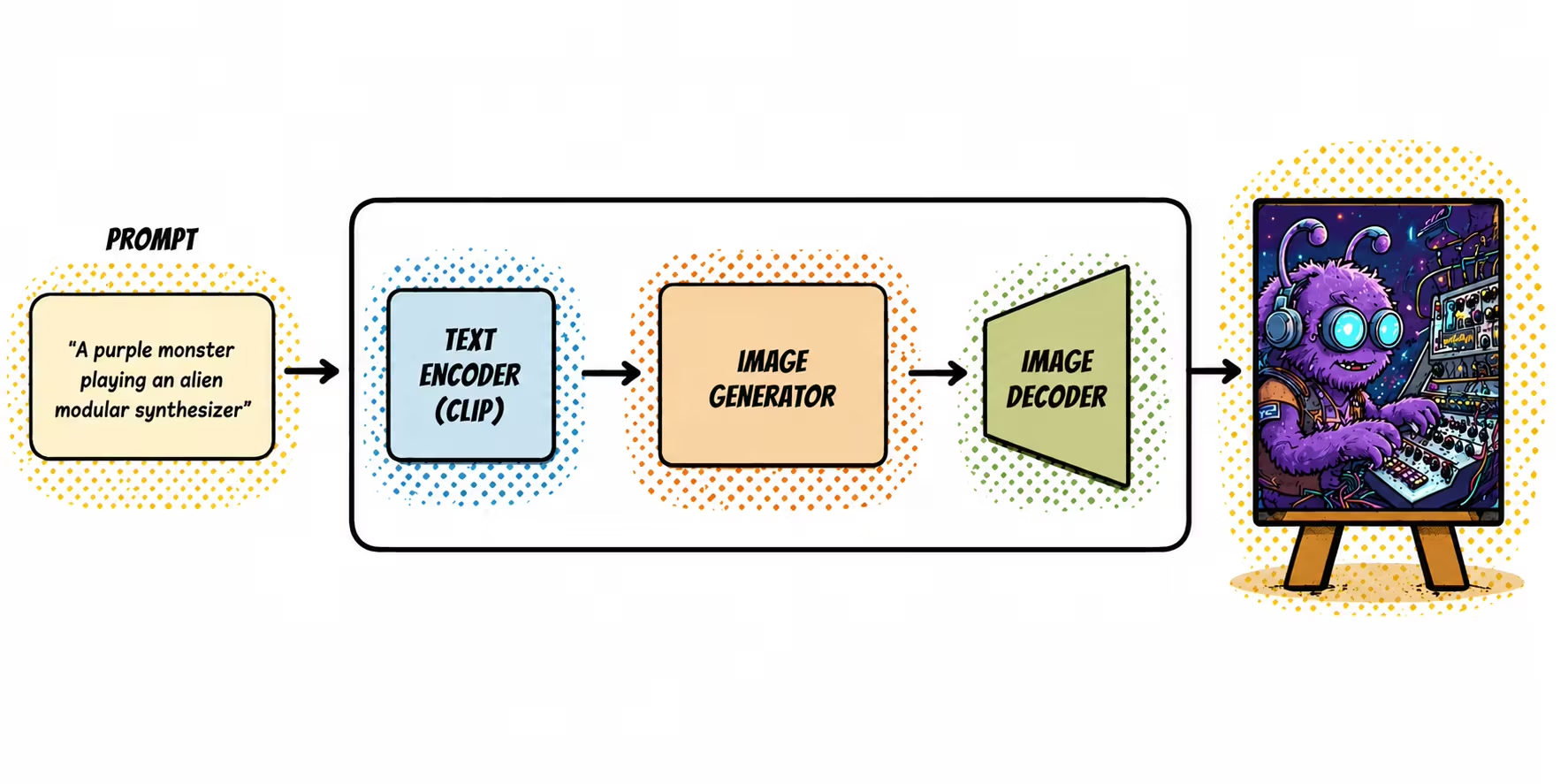
We can think of Stable Diffusion as three main blocks:

1. Text encoder: converts the text prompt into a numerical representation.
2. Image generator: generates a latent representation of the image guided by the text.
3. Image decoder: reconstructs the latent representation into the target image dimension.

Text encoder: CLIP

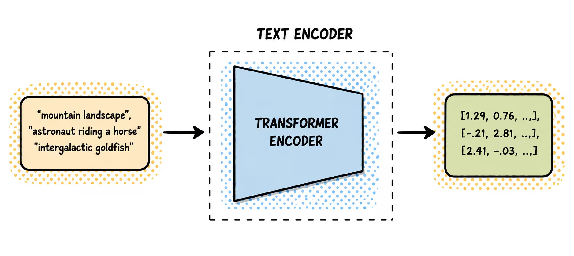
First, the model needs to convert prompts into vectors that a neural network can use.

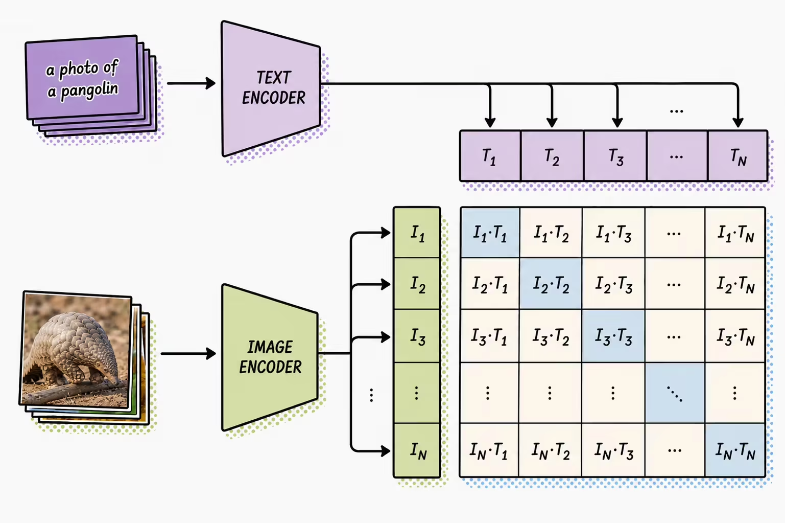
In the original Stable Diffusion, this block is CLIP's text encoder^{[radford2021learning]}. CLIP jointly trains an image encoder and a text encoder to learn representations where an image and its description end up close together in vector space.

During training, image-text pairs are passed through their respective encoders and the embeddings are compared using cosine similarity. At the start, the similarity will be low, even if the text correctly describes the image, simply because the vector spaces of each encoder are different. What is then done is to update the weights of both networks so that, next time, the resulting embeddings are similar.

By repeating this operation, by the end of training the encoders end up producing embeddings in which, for example, an image of a pangolin and the phrase "a photo of a pangolin" end up in similar regions of the latent space.

The text encoder is used to convert the prompt into a sequence of embeddings that contain contextual representations of the tokens. The generator will use it to guide the appearance of objects, styles, and relationships.

Example: if the prompt says "a dog with sunglasses on the beach", the text encoder generates a representation that will help the image generator know that concepts like dog, sunglasses, beach, outdoor light, sand, etc., should appear.

Image generator

The name "image generator" can be misleading because, in the Stable Diffusion family, this component does not produce pixels directly, but rather a matrix in latent space.

The core block is a U-Net. This network receives:

• a noisy latent $z_t$
• the timestep $t$
• the textual conditioning $c$ produced by CLIP

And predicts the noise that should be subtracted:

$$\epsilon_\theta(z_t, t, c)$$

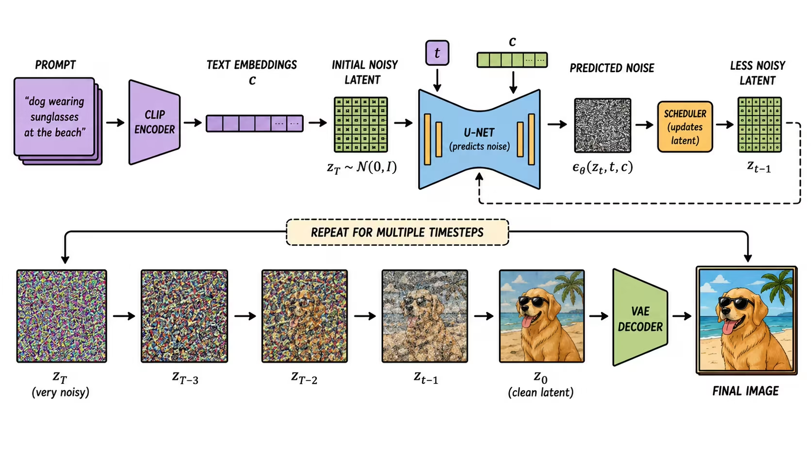
Then, a scheduler uses that prediction to compute a slightly less noisy latent:

$$z_t \rightarrow z_{t-1}$$

This process is repeated many times until a clean latent $z_0$ is obtained. This is not a visible image, so it is passed through the decoder of a VAE to convert it into pixels, $\hat{x} = D_{\text{VAE}}(z_0)$.

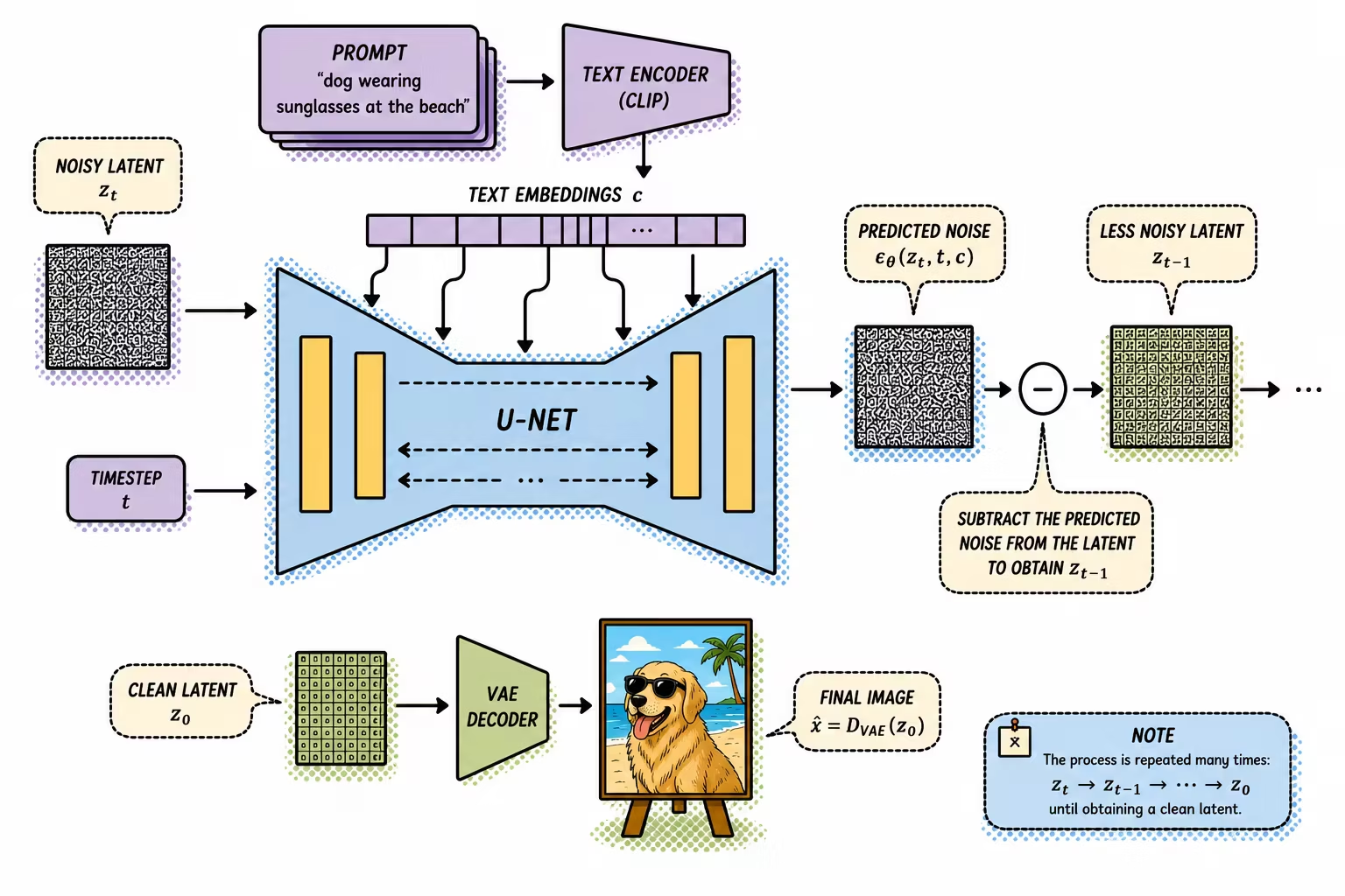
The U-Net uses cross-attention mechanisms to mix the visual information of the latent with the textual information of the prompt. Thanks to this, the model can decide which parts of the image should attend to which parts of the text.

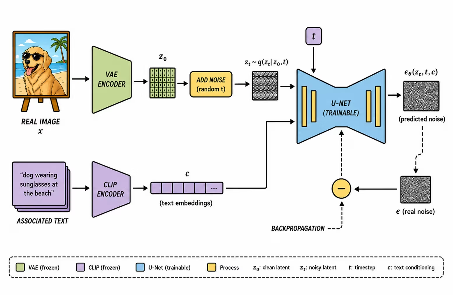
Training

During training, the model mainly learns to remove noise in the latent space.

The typical process is:

1. A real image $x$ and its associated text are taken.
2. The image is encoded with the VAE's encoder to obtain a latent $z_0$.
3. The text is encoded with CLIP to obtain the conditioning $c$.
4. A random timestep $t$ is chosen.
5. Noise is added to the latent $z_0$ to obtain $z_t$.
6. The U-Net receives $(z_t, t, c)$ and predicts the added noise.
7. The real noise is compared with the predicted noise.

The loss is the same $\mathcal{L}_{\mathrm{simple}}$ we just defined, but applied in the latent space and conditioned on the text:

$$\mathcal{L}_{\mathrm{simple}}^{\mathrm{latent}}(\theta) = \mathbb{E}_{z_0, \epsilon, t, c} \left[ \left\| \epsilon - \epsilon_\theta(z_t, t, c) \right\|^2 \right]$$

In many implementations, the VAE and the text encoder are already pretrained, so they are kept frozen. The trainable part consists of the U-Net's parameters for the denoising process.

Inference

Here we want to use the already-trained model to generate a new image.

The typical flow is:

1. We write a prompt.
2. CLIP converts the prompt into text embeddings $c$.
3. We sample a random initial latent $z_T \sim \mathcal{N}(0, I)$.
4. The U-Net predicts the noise in the current latent, conditioned on $c$.
5. The scheduler subtracts the predicted noise from the latent to make it slightly less noisy.
6. We repeat steps 4 and 5 for several timesteps.
7. The decoder converts the final latent $z_0$ into an image.

Relationship to Flow Matching

Diffusion models and Flow Matching are closely related. Both start from a simple distribution, usually Gaussian noise, and learn to transform it into a target distribution. The most common way of presenting them differs in which parametrization the model uses to express that same objective, although, as we'll see, all of them are convertible into one another.

In diffusion, the model learns to predict the noise:

$$\epsilon_\theta(x_t, t)$$

That is, it receives a noisy sample $x_t$ and predicts which part of that sample corresponds to the added noise.

In Flow Matching, the model learns a velocity:

$$v_\theta(x_t, t)$$

That is, it receives an intermediate point $x_t$ and predicts in which direction it should move to advance from the initial distribution toward the target distribution.

During training

In diffusion, we construct noisy examples by adding known noise to real data:

$$x_t = \sqrt{\bar{\alpha}_t}x_0 + \sqrt{1 - \bar{\alpha}_t}\epsilon$$

Since we know $\epsilon$, we train the network to predict that noise.

In Flow Matching, we construct intermediate points between an initial sample $z$ and a data point $x$:

$$x_t = (1 - t)z + tx$$

And we train the network to predict the velocity that would follow that path:

$$u_t = x - z$$

In both cases we build a supervised problem: we artificially generate an intermediate state and we know what the correct answer should be. In diffusion this target can also be expressed as a score, a clean sample $x_0$, or a velocity $v$.

These parametrizations are not independent: given $x_t = \sqrt{\bar{\alpha}_t}\,x_0 + \sqrt{1 - \bar{\alpha}_t}\,\epsilon$, they are related by

$$x_0 = \frac{x_t - \sqrt{1-\bar{\alpha}_t}\,\epsilon}{\sqrt{\bar{\alpha}_t}}, \qquad s(x_t,t) = -\frac{\epsilon}{\sqrt{1-\bar{\alpha}_t}}, \qquad v = \sqrt{\bar{\alpha}_t}\,\epsilon - \sqrt{1-\bar{\alpha}_t}\,x_0.$$

Given $x_t$ and any one of the four quantities (noise $\epsilon$, score $s$, clean data $x_0$, or velocity $v$), the others can be obtained without retraining the model. They are different parametrizations of the same training objective.

During generation

In diffusion, we start from noise and apply denoising steps:

$$x_T \rightarrow x_{T-1} \rightarrow \cdots \rightarrow x_0$$

In Flow Matching, we start from noise and follow a velocity field:

$$\frac{dx_t}{dt} = v_\theta(x_t, t)$$

Generation also proceeds from noise to data, but the mathematical starting point changes. Diffusion can be implemented as a stochastic chain or via its probability-flow ODE; Flow Matching directly defines and learns a velocity field over a probability path. The two frameworks are closely related.