Probabilistic Machine Learning

There are many types of generative models. At a high level we can distinguish between:

• Probabilistic Graphical Models (PGM): they represent, by means of a graph, the probabilistic relationships between observed (and/or latent) variables, showing how a joint distribution decomposes and what conditional independences exist between them.
• Deep Generative Models (DGM): they use deep neural networks to model or generate data distributions. Some incorporate latent variables $z$, although this is not a requirement common to all families.

Of course, many hybrids are possible. From here on we'll focus on DGMs.

The main types of DGM are variational autoencoders (VAE), generative adversarial networks (GAN), autoregressive models (ARM), flow-based models and diffusion models.

These models can be classified according to the following criteria:

• Density: models that can estimate the probability density function $p(x)$. For example, GANs model the data distribution implicitly, so they cannot.
• Sampling: models that can generate new samples from the modeled distribution. Models like VAEs and GANs allow fast sampling. However, ARMs, diffusion models or normalizing flows are (generally) slow to sample from.
• Training: what kind of method is used to estimate the parameters? For some models (like ARM and flows), an exact maximum likelihood estimation (MLE) can be performed. For other models it isn't so simple. For example, in the case of VAEs a lower bound on the likelihood is maximized.
• Latents: does the model use a latent vector $z$ to generate $x$? And, if so, does it have the same size as $x$ or is it a compressed representation? For example, ARMs don't use latent representations; flows and diffusion do, but they aren't compressed representations.
• Architecture: what kind of neural network can be used? Are there any restrictions? In the case of flows, for example, only invertible neural networks can be used, where each layer has a tractable Jacobian.

Here's a brief summary of how the main models work. If this is the first time you're seeing this diagram, don't worry if you don't understand it yet. I recommend coming back to it as we move forward.

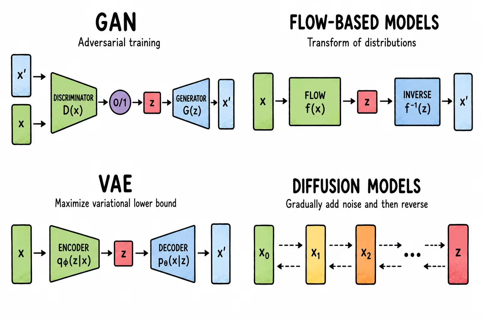
In the coming chapters we'll make use of probabilistic notation. If it's something you already know well, you can skip straight to the first chapter. If not, in the rest of this article we'll do a quick review of probability.

Probability

There are two different interpretations of probability:

• Frequentist: probabilities represent frequencies of events that can occur multiple times.

  Example: the probability of rolling a 6 if you roll a die 600 times. We expect the number 6 to come up approximately 100 times. It's assumed that conditions are stable and that, if you repeat the experiment many times, the result will converge toward a fixed frequency (in this case 1/6).

• Bayesian: probability is used to quantify uncertainty/ignorance about something. The Bayesian interpretation can be used to model uncertainty about one-off events that don't have long-run frequencies.

  Example: say we want to calculate the probability that the polar ice cap will melt in 2030. This event will either happen or not, but it can't happen repeatedly. Nevertheless, we should be able to quantify our uncertainty about this event.

From here on we'll adopt the Bayesian interpretation. Fortunately, the basic rules of probability theory are the same regardless of which interpretation is adopted.

Basic rules

Probability of an event

We define an event $A$ as a state that either holds or doesn't. For example, $A$ can be the event "it will rain tomorrow" or "it rained yesterday". The expression $\Pr(A)$ denotes the probability with which the event $A$ is believed to be true. We require $0 \leq \Pr(A) \leq 1$, where $\Pr(A) = 0$ means the event won't occur and $\Pr(A) = 1$ means it will.

Random variables

Suppose $X$ represents some unknown quantity, like the face a die will land on when rolled. If the value of $X$ is unknown and/or can change, we call it a random variable. The set of possible values, denoted $\mathcal X$, is known as the sample space or state space. An event is a set of outcomes from a given sample space.

For example, if $X$ represents the face of a die, $\mathcal X = \{1, 2, \dots, 6\}$. The event "seeing a 1" is denoted $X = 1$, the event "seeing an odd number" is denoted $X \in \{1, 3, 5\}$, the event "seeing a number between 1 and 3" is denoted $1 \leq X \leq 3$, etc.

Discrete random variables

If the sample space $\mathcal X$ is countable (finite or countably infinite), $X$ is called a discrete random variable. Example: rolling a die, the number of customers entering a store, the number of heads in 5 coin flips...

The function that describes the probability distribution of discrete random variables is called the probability mass function or pmf:

$$p(x) = \Pr(X = x),$$

where $x$ is a possible value within the sample space.

Continuous random variables

If $X \in \mathbb{R}$, it's called a continuous random variable. Example: time, weight, temperature...

In this case, you can't create a finite set of the different possible values the variable can take. However, they can be divided into different intervals.

Here, unlike the PMF, which tells us the probability of an exact value occurring, we use the cumulative distribution function or cdf, which tells us the probability of that value or any smaller one occurring:

$$P(x) = \Pr(X \leq x)$$

Note that an uppercase $P$ is used to represent the cdf.

Using this, we can calculate the probability of being within any interval:

$$\Pr(a < X \leq b) = P(b) - P(a)$$

The function that describes the probability distribution of continuous random variables is called the probability density function or pdf, which coincides with the derivative of the cdf:

$$p(x) = \frac{d}{dx} P(x)$$

• The PMF (discrete) measures "bars" (exact points).
• The PDF (continuous) measures "areas" (intervals).

Given a pdf, we can calculate the probability that a continuous variable falls within a finite interval as:

$$\Pr(a < X \leq b) = \int_{a}^{b} p(x)\, dx = P(b) - P(a)$$

Example: Waiting time at a bus stop

Imagine the waiting time (in minutes) for the bus follows a uniform distribution between 0 and 10 minutes. Its PDF is constant: $p(x)=1/10$ for $0 \leq x \leq 10$, and 0 otherwise. If we want to know the probability that the bus arrives between minute 2 and minute 5, $\Pr(2 < X \leq 5)$, we use the integral of the PDF:

$$\Pr(2 < X \leq 5) = \int_{2}^{5} \frac{1}{10} \, dx$$

We calculate the integral:

$$\left[ \frac{1}{10}x \right]_{2}^{5} = \frac{5}{10} - \frac{2}{10} = \frac{3}{10} = 0.3$$

Therefore, there is a 30% probability that the bus arrives within that time interval.

Statistics

• Mean ($\mu$): arithmetic average, represents the value you would get if you could distribute the total of the data equally among all the elements.
• Variance ($\sigma^2$): a measure of the spread of a distribution, it measures how far, on average, the values deviate from the mean. Since it squares the differences, its units are also squared (for example, if you measure in meters, the variance will be in square meters).
• Standard deviation ($\sigma$): the square root of the variance. It fixes the "problem" with the variance. It gives an idea of how far the data deviates from the average in the original units.

Bayesian inference

The term "inference" refers to the act of generalizing from sample data, usually with some degree of confidence. The term "Bayesian" is used to refer to inference methods that represent that confidence using probability theory and Bayes' theorem.

Bayes' theorem is a formula for calculating the probability distribution over possible values of an unknown quantity $H$ given observed data $Y$:

$$p(H \mid Y) = \frac{p(Y \mid H)\, p(H)}{p(Y)}$$

• $p(H)$ represents what is known about the possible values of $H$ before seeing any data; this is the prior distribution.
• $p(Y \mid H)$ represents the distribution over the possible outcomes $Y$ we expect to see given $H$; this is the observation distribution.
• If we fix it at the value $Y=y$ corresponding to the actual observations, but treat it as a function of $H$ (rather than of $Y$), we get the likelihood function, $\mathcal{L}(H) = p(Y=y \mid H)$.

Multiplying the prior distribution $p(H)$ by the likelihood function $p(Y \mid H)$ for each $h$ gives the unnormalized joint distribution $p(H, Y)$. It can be turned into a normalized distribution by dividing by $p(Y)$, which is known as the marginal likelihood (we'll see this later).

By normalizing the joint distribution, we get the posterior distribution, $p(H \mid Y)$, which represents what is known about the distribution after seeing evidence. In other words:

$$\text{posterior} \propto \text{prior} \times \text{likelihood}$$

Example: test for a rare disease

Imagine you want to know whether a patient has a rare disease (Hypothesis $H$) that affects only 1% of the population.

1. Prior distribution, $p(H)$: before taking the test, the probability that the patient is sick is 0.01.
2. Likelihood, $p(Y \mid H)$: the sensitivity is $p(Y=\text{pos}\mid H=\text{sick})=0{,}99$ and the false positive rate is $p(Y=\text{pos}\mid H=\text{healthy})=0{,}05$.
3. Posterior distribution, $p(H \mid Y)$: once a positive result is observed, we want to calculate the probability that the patient is actually sick.

You might confuse the 99% sensitivity with the probability of being sick after a positive result. However, applying Bayes' theorem we get:

$$p(H = \text{sick} \mid Y = \text{pos}) = \frac{p(Y = \text{pos} \mid H = \text{sick}) \cdot p(H = \text{sick})}{p(Y = \text{pos})}$$

Where:

• Prior $p(H = \text{sick}) = 0.01$ (only 1% of the population is sick).
• Likelihood $p(Y = \text{pos} \mid H = \text{sick}) = 0.99$ (the test detects 99% of sick people).
• False positives $p(Y = \text{pos} \mid H = \text{healthy}) = 0.05$ (the test is wrong for 5% of healthy people).

Step 1: Calculate the total probability of a positive result $p(Y = \text{pos})$

A positive can be a true positive (sick person who tests positive) or a false positive (healthy person who tests positive):

$$p(Y = \text{pos}) = (\text{Sensitivity} \times \text{Prevalence}) + (\text{False positive rate} \times \text{Healthy population})$$ $$p(Y = \text{pos}) = (0.99 \times 0.01) + (0.05 \times 0.99)$$ $$p(Y = \text{pos}) = 0.0099 + 0.0495 = 0.0594$$

Step 2: Calculate the Posterior

Now we substitute into Bayes' formula:

$$p(H = \text{sick} \mid Y = \text{pos}) = \frac{0.99 \cdot 0.01}{0.0594} \approx 0.166$$

Conclusion: Although the test has a sensitivity of 99%, the probability that the patient is sick after testing positive is approximately 16.7%. The low prevalence (the prior) "pulls" the result down very strongly. The number of healthy people in the population is so large that the 5% false positive rate outnumbers the true positives. This example shows that, in Bayesian inference, the observed data isn't the only thing that determines reality; our initial belief about how rare the event is plays a fundamental role.

Probability distributions

There is a wide variety of probability distributions used for different types of models. At this link you can explore some of the most commonly used ones interactively.

A generative model learns a distribution over the data, $p(x)$ for $x \in \mathcal{X}$, or a joint distribution $p(x,y)$ when several variables are involved. In the following chapters we'll see different ways of representing, approximating and sampling from it.