Flow-based Models

Generative models differ in how they relate to the density of the data $p(x)$. GANs are implicit density models: they do not compute or optimize any likelihood, they only learn to sample through an adversarial game. VAEs are likelihood-based models, but their marginal likelihood is intractable and is optimized via a lower bound (the ELBO). Flow-based models, on the other hand, allow this density to be computed exactly and tractably.

As we already saw, a typical generative model with latent variables is defined by:

$$p(x) = \int p(x \mid z)\, p(z)\, dz,$$

and computing $p(x)$ is intractable because it is practically impossible to iterate over all values of $z$.

Flow-based models approach this problem through invertible transformations of distributions. There are two major families: classical normalizing flows, which apply a discrete sequence of invertible transformations, and continuous normalizing flows (CNF), where the transformation is defined as the solution of an ordinary differential equation (ODE); we will look at the latter further on.

A good estimate of $p(x)$ makes it possible to efficiently carry out many tasks, such as sampling new, unobserved but realistic data points (data generation), inferring latent variables, or filling in incomplete data samples. Their use for detecting out-of-distribution (OOD) data has also been explored.

Normalizing flows

Since we use backpropagation to train deep learning models, we expect the posterior probability distribution $p(z \mid x)$ to be simple enough that its derivative can be computed easily and efficiently. This is why the Gaussian distribution is usually used in latent-variable generative models, even though most real-world distributions are much more complicated than the Gaussian.

In a normalizing flow, to approximate the real distribution we start from a simple distribution $p_0(z_0)$, to which a series of invertible transformations is applied to turn it into a complex one $p_K(z_K)$. The variable $z_i$ is repeatedly replaced by the new $z_{i+1}$ to finally obtain a probability distribution matching the final target variable.

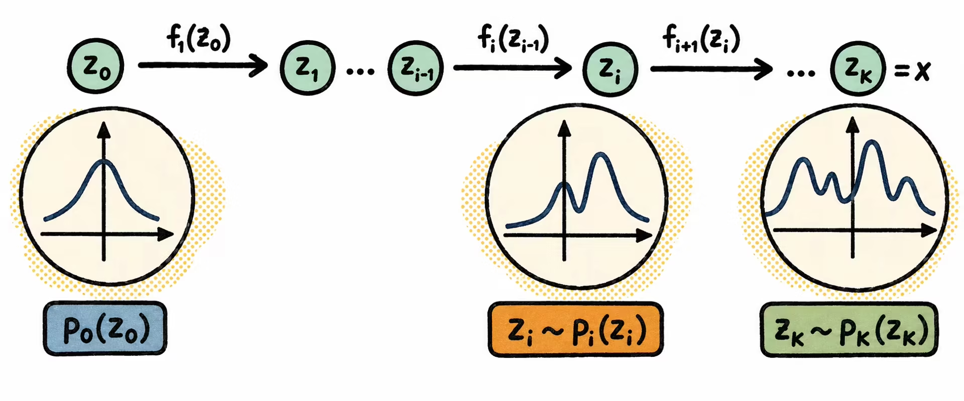
Both the forward transformation and its inverse can be computed exactly. This makes density estimation possible. To do this, two things must be taken into account:

• The density of the inversely transformed sample: to obtain the transformed sample, the sequence of inverse transformations is applied to the original sample. Then, the density of this transformed sample is evaluated under the original simple distribution. That is, we check whether the resulting transformation is a Gaussian.
• The change of volume due to the transformations: as the transformations are carried out, the sample space is distorted. The change of volume is calculated by multiplying the absolute values of the determinants of the Jacobian matrices of each transformation.

By multiplying these two values (the density of the transformed sample and the change of volume), we obtain the density of the original sample under the complex distribution.

Applications

The most direct applications of normalizing flows are:

• Density estimation: to compute the exact density of the data (the one assigned by the model). They can be applied to fit multimodal densities to observed data. They can also be used as hybrid models that model the joint density of inputs and targets $p(x, y)$, unlike classification models, which only model $p(y \mid x)$, and density models, which only model $p(x)$. This is useful for tasks such as anomaly detection.
• Data generation: for different data modalities, including images, video, audio, text, and structured objects such as graphs.
• Inference: instead of blindly trying combinations in a simulator or digital twin until finding which parameters are compatible with an observed result, the flow learns to take the reverse path: starting from an observation, it approximates the posterior distribution over the parameters that could have generated it, without needing to run through the simulator thousands of times. This approach saves months of computation in fields such as cosmology^{[alsing2019fast]} and computational neuroscience^{[goncalves2019training]}.

Basic linear algebra concepts

Jacobian matrix

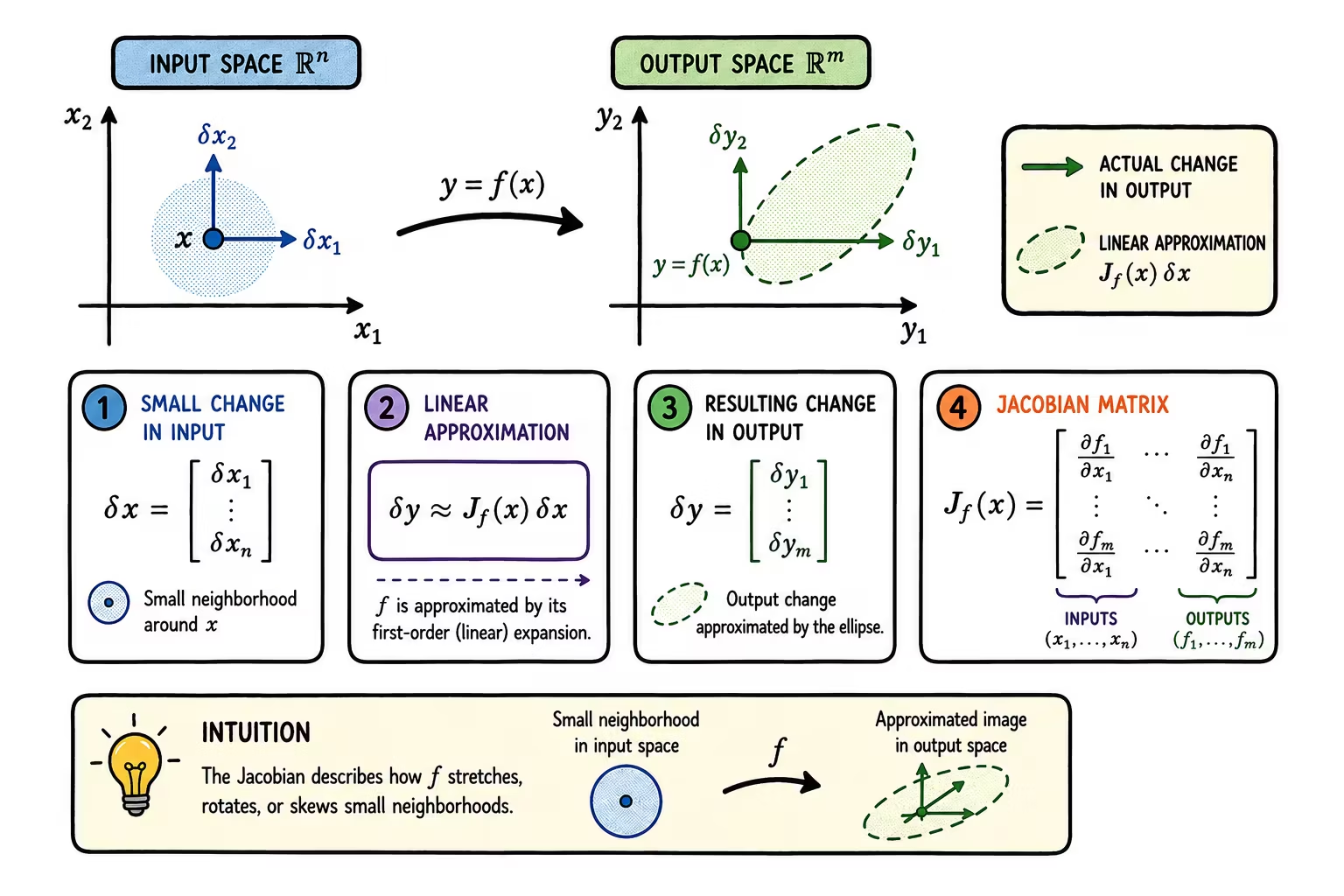
Given a function mapping an $n$-dimensional input vector to an $m$-dimensional output vector, the matrix of all the first-order partial derivatives of this function is called the Jacobian matrix:

$$\mathbf{J} = \begin{bmatrix} \dfrac{\partial f_1}{\partial x_1} & \cdots & \dfrac{\partial f_1}{\partial x_n} \\ \vdots & \ddots & \vdots \\ \dfrac{\partial f_m}{\partial x_1} & \cdots & \dfrac{\partial f_m}{\partial x_n} \end{bmatrix}$$

It can be understood as a translator from one vector space to another.

Determinant

The absolute value of the determinant (which only exists for square matrices) can be thought of as a measure of "how much multiplication by the matrix expands or contracts space."

The determinant of a square matrix $M$ detects whether it is invertible:

• if $\det(M) = 0$ then it is not invertible (a singular matrix with linearly dependent rows or columns; or any row or column that is all 0);

• if $\det(M) \neq 0$, then $M$ is invertible.

The determinant of a product is equivalent to the product of the determinants: $\det(AB) = \det(A)\det(B)$.

Change of variables theorem

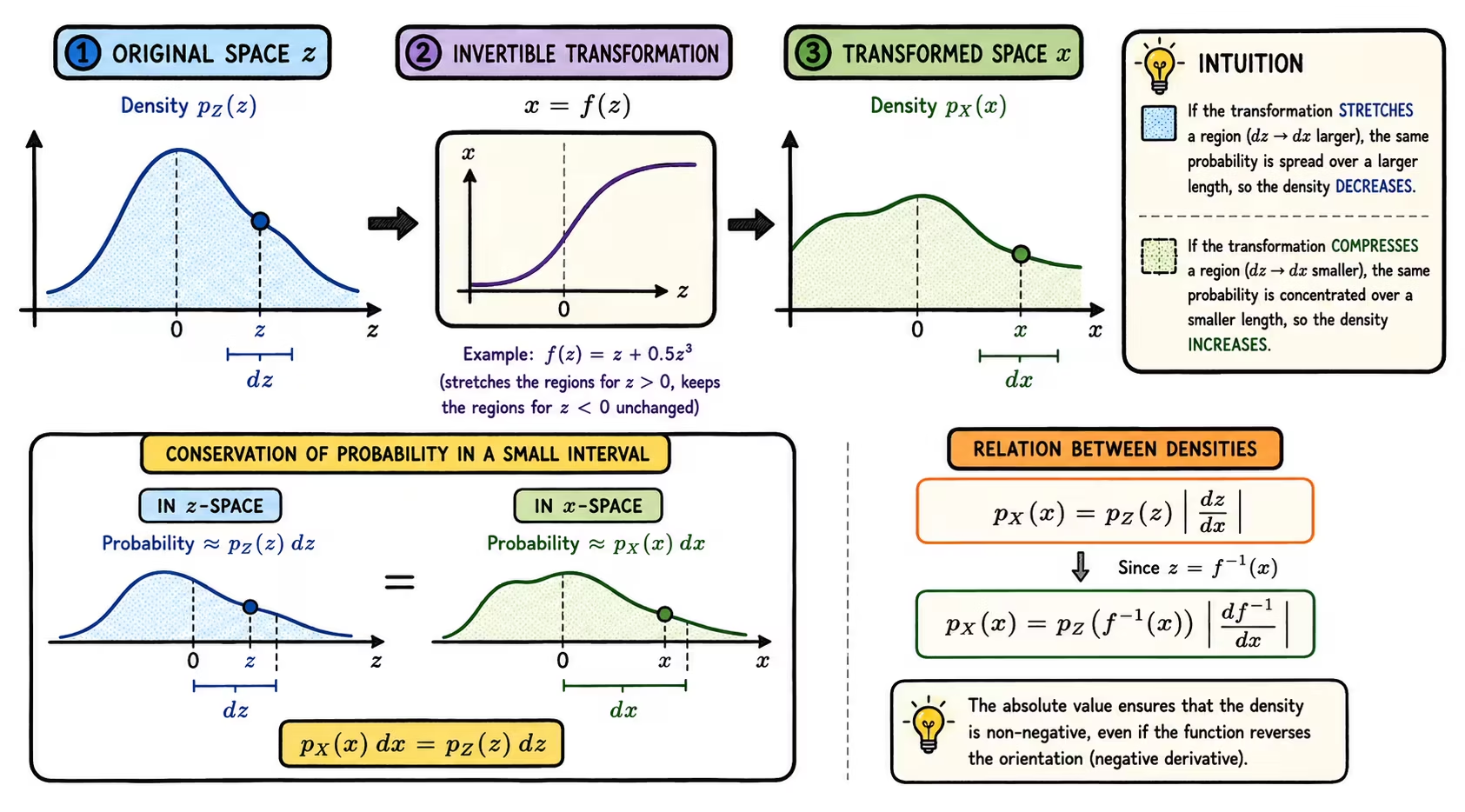
When we transform a random variable, its probability does not change, but the space it lives in can stretch or compress.

Imagine a simple variable $z$ with known density $p_Z(z)$, for example a Gaussian. Now we apply an invertible function:

$$x = f(z)$$

Since $f$ is invertible, if we know a value of $x$ we can also recover the value of $z$ that produced it:

$$z = f^{-1}(x)$$

The question is: if we know the density in the original space, $p_Z(z)$, how do we compute the density in the new space, $p_X(x)$?

At first glance, one might think it is:

$$p_X(x) = p_Z(f^{-1}(x))$$

This tells us where $x$ comes from, BUT the transformation may have changed the size of the regions of space.

In one dimension, we can think of it in terms of small intervals. A little piece around $z$ has length $dz$. After applying the transformation, that piece becomes another one around $x$ with length $dx$.

The probability inside both pieces must be the same:

$$p_X(x)\, dx = p_Z(z)\, dz$$

Rearranging:

$$p_X(x) = p_Z(z) \left| \frac{dz}{dx} \right|$$

And since $z = f^{-1}(x)$:

$$p_X(x) = p_Z(f^{-1}(x)) \left| \frac{df^{-1}}{dx} \right|$$

The absolute value appears because a density cannot be negative. If the function flips the axis, for example from left to right, the derivative can be negative, but the size-change factor remains positive.

In several dimensions the same thing happens, but the "little pieces" are no longer intervals, but small areas, volumes, or hypervolumes. This is where the Jacobian determinant comes in:

$$p_X(x) = p_Z(f^{-1}(x)) \left| \det J_{f^{-1}}(x) \right|$$

Where $J_{f^{-1}}(x)$ is the Jacobian matrix of the inverse function. Its determinant measures how much the volume locally expands or contracts when going from $x$ back to $z$.

This is also often written using the forward transformation $f$:

$$p_X(x) = p_Z(z) \left| \det J_f(z) \right|^{-1}$$

This form is equivalent. If $f$ stretches the volume by a factor of $3$, then the density is divided by $3$. If it compresses it by a factor of $3$, then the density is multiplied by $3$.

Application to normalizing flows

A normalizing flow does not perform a single transformation, but a chain of invertible transformations:

$$z_0 \xrightarrow{f_1} z_1 \xrightarrow{f_2} z_2 \xrightarrow{f_3} \cdots \xrightarrow{f_K} z_K = x$$

We normally start with a simple distribution:

$$z_0 \sim p_0(z_0)$$

Then we apply transformations until we reach a sample that looks like real data:

$$x = z_K = f_K \circ f_{K-1} \circ \cdots \circ f_1(z_0)$$

This is used to generate data: we sample a simple $z_0$ and progressively transform it to obtain $x$.

But the interesting thing about flows is that we can also take the reverse path to compute the exact density of a data point $x$:

$$x = z_K \xrightarrow{f_K^{-1}} z_{K-1} \xrightarrow{f_{K-1}^{-1}} \cdots \xrightarrow{f_1^{-1}} z_0$$

Once we have $z_0$, its density is easy to compute because it belongs to the initial distribution. All that remains is to correct for all the volume changes that occurred along the way.

For a single transformation:

$$z_i = f_i(z_{i-1})$$

Applying the change of variables theorem:

$$p_i(z_i) = p_{i-1}(z_{i-1}) \left| \det J_{f_i}(z_{i-1}) \right|^{-1}$$

This equation says:

• the density after the transformation depends on the density before the transformation
• if the transformation expands the space, the density decreases
• if the transformation compresses the space, the density increases

As we mentioned in the GAN chapter, in machine learning we usually work with logarithms of probabilities because:

• products of many small numbers tend to zero
• products become sums, which are easier to optimize

Taking logarithms:

$$\log p_i(z_i) = \log p_{i-1}(z_{i-1}) - \log \left| \det J_{f_i}(z_{i-1}) \right|$$

If we repeat this for the $K$ transformations of the flow, we obtain:

$$\log p_X(x) = \log p_0(z_0) - \sum_{i=1}^{K} \log \left| \det J_{f_i}(z_{i-1}) \right|$$

This is the central formula of normalizing flows.

It reads as follows:

• $\log p_X(x)$: the log-density of the real data point we want to evaluate
• $\log p_0(z_0)$: the log-density of the corresponding point in the simple distribution
• $\sum_i \log |\det J_{f_i}|$: the accumulated correction for all the volume changes introduced by the transformations

The path traveled by the random variables $z_i = f_i(z_{i-1})$ is the flow. The complete chain of successive distributions is what we call a normalizing flow.

Models based on Normalizing flows

Some popular normalizing flow architectures are Real NVP^{[dinh2016density]}, Masked Autoregressive Flows^{[papamakarios2017masked]}, Glow^{[kingma2018glow]} (by Kingma $\rightarrow$ author of the original VAE paper and creator of the Adam optimizer), and SurVAE^{[nielsen2020survae]}.

The differences between these architectures lie in the transformations they apply and in specific network designs, but they all share the common goal of transforming a simple distribution into a more complex one.

Advantages and disadvantages

Flow Matching

As we have seen, normalizing flows build the model as a chain of invertible transformations:

$$z_0 \xrightarrow{f_1} z_1 \xrightarrow{f_2} \cdots \xrightarrow{f_K} x$$

Flow Matching starts from a similar idea, but instead of asking:

What invertible transformations can I design to turn noise into data?

it asks:

What direction should each point follow to move from a simple distribution to the target distribution?

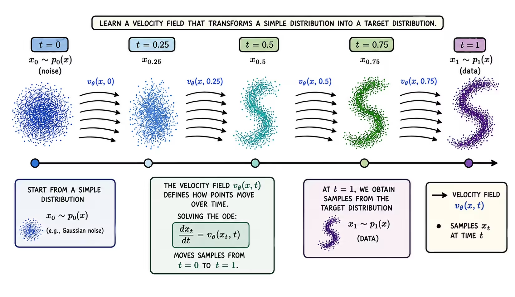
In this way, what Flow Matching learns is a velocity field.

Imagine we have many noise points, for example samples from a Gaussian, and many real points, for example images. We want to gradually move the noise points until they end up resembling the real data.

To describe this movement we introduce a time variable:

$$t \in [0, 1]$$

When $t = 0$, we are at the simple distribution:

$$x_0 \sim p_0$$

When $t = 1$, we want to be at the data distribution:

$$x_1 \sim p_{\text{data}}$$

In between we have intermediate points $x_t$. The model learns a function:

$$v_\theta(x_t, t)$$

This function receives two things:

• the current point $x_t$
• the current time $t$

And returns a vector indicating where that point should move at that instant.

Training

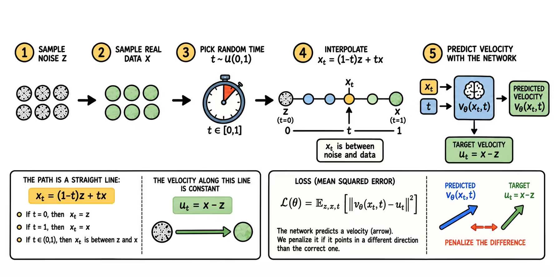
To train the model we need to know what a good velocity would be at different intermediate points. To do this, we can pair a noise point $z$ with a real data point $x$ and draw a line between them:

$$x_t = (1 - t)z + tx$$

This equation represents an interpolation where:

• if $t = 0$, then $x_t = z$
• if $t = 1$, then $x_t = x$
• if $t$ is between 0 and 1, then $x_t$ is between the noise and the data

If the path is a straight line, the velocity that leads from $z$ to $x$ is:

$$u_t = x - z$$

Therefore, during training we can do the following:

1. Take a noise sample $z$
2. Take a real data point $x$
3. Choose a random time $t$ between 0 and 1
4. Construct the intermediate point $x_t = (1 - t)z + tx$
5. Ask the network to predict the correct velocity $u_t = x - z$

The loss function can be written as:

$$\mathcal{L}(\theta) = \mathbb{E}_{z, x, t} \left[ \left\| v_\theta(x_t, t) - u_t \right\|^2 \right]$$

The idea is fairly direct: the network predicts an arrow, which is penalized if it points in a direction different from the one it should.

Sample generation

Once the model is trained, generating a sample consists of solving an ordinary differential equation (ODE):

$$\frac{dx_t}{dt} = v_\theta(x_t, t)$$

This roughly means: "update $x_t$ following the velocity predicted by the network at each instant."

In practice:

1. We sample an initial noise point $x_0 \sim p_0$
2. We use the network to know where to move it
3. We take a small step in that direction
4. We repeat the process from $t = 0$ to $t = 1$

At the end we obtain $x_1$, which should look like a sample from the data distribution.

Difference from Normalizing Flows

Normalizing flows and Flow Matching share the same intuition: both transform a simple distribution into a complex distribution. The difference lies in how they do it.

In normalizing flows:

• we use a finite sequence of invertible transformations
• we compute how the density changes with Jacobian determinants
• we can evaluate the density assigned by the model

In Flow Matching:

• we learn a continuous velocity field
• we generate data by following a trajectory from noise to data
• we do not need to manually design invertible layers with easy determinants

This is why Flow Matching is appealing: it allows the use of more flexible neural networks and training them with a relatively simple regression loss.

Continuous Normalizing Flows

Until now, when we talked about Normalizing Flows we were referring to discrete flows. However, there are also continuous flows, where, instead of applying a chain of discrete layers, the transformation is modeled as a continuous process in time governed by an ODE.

The problem is that training these flows required "simulating" the ODE forward and backward within each optimization step (known as simulation-based training or the use of Neural ODEs), which is computationally exhausting and very slow.

In this sense, the training reformulation proposed by Flow Matching (direct, linear probability paths and a simple regression loss) makes it possible to solve this problem during training: it is no longer necessary to simulate the ODE at every optimization step.

Optimal Transport

Once the central idea of Flow Matching is understood, it makes sense to talk about Optimal Transport as a way of choosing better paths between the initial distribution and the data distribution.

The intuition behind Optimal Transport is to transform one distribution into another at the lowest possible cost.

In Flow Matching this comes up when we construct paths between noise points and real points. If we pair points at random, the trajectories can cross a lot or take unnecessary detours. If we use the idea of optimal transport, we try to pair points in a more coherent way.

This is why variants such as Optimal Transport Flow Matching or OT-CFM appear in the literature. The original paper Flow Matching for Generative Modeling^{[lipman2022flow]} already highlights the use of optimal-transport-based paths as a particularly interesting option, and later works such as Improving and Generalizing Flow-Based Generative Models with Minibatch Optimal Transport^{[tong2023improving]} use optimal transport on mini-batches to build more useful pairings during training.

What matters is not to confuse the levels:

• Flow Matching: learns a velocity field that moves samples from noise to data.
• Optimal Transport: can help define more efficient paths or pairings for training that velocity field.

Relationship with diffusion models

Flow Matching is closely related to diffusion models, because both describe a process that connects noise with data.

In diffusion, one usually learns to invert a stochastic process that adds noise. The same model can parameterize noise, score, $x_0$, or velocity, and these parameterizations can be converted into one another for a given noise path. For example, for the linear path used in Flow Matching, $x_t = (1-t)x_0 + t\varepsilon$ with $\varepsilon\sim\mathcal N(0,I)$:

$$\varepsilon = \frac{x_t - (1-t)x_0}{t}, \qquad x_0 = \frac{x_t - t\,\varepsilon}{1-t}, \qquad s(x_t,t) = -\frac{\varepsilon}{t}, \qquad v(x_t,t) = \varepsilon - x_0.$$

Given $x_t$ and any one of the four quantities (noise $\varepsilon$, score $s$, $x_0$, or velocity $v$), the others can be obtained without retraining the model. Other (nonlinear) noise paths give rise to analogous relationships but with different coefficients, as we will see in the next chapter.

In Flow Matching, the velocity field that transports samples from noise to data is learned directly.

Therefore, both frameworks are closely related: they differ in the objective and in how the path is specified, as we will see in the next chapter.