Efficiency and cost reduction
Today's generative models can contain billions of parameters. Training, adapting, and serving them requires memory to store their weights and activations, and computing power to carry out the operations.
There is no single way to reduce this cost. In this chapter we will look at three complementary strategies:
- Distillation: training a smaller model to reproduce the behavior of a more capable one.
- Quantization: representing weights and, in some cases, activations with fewer bits.
- LoRA: adapting a pretrained model by updating only a small number of parameters.
Knowledge distillation
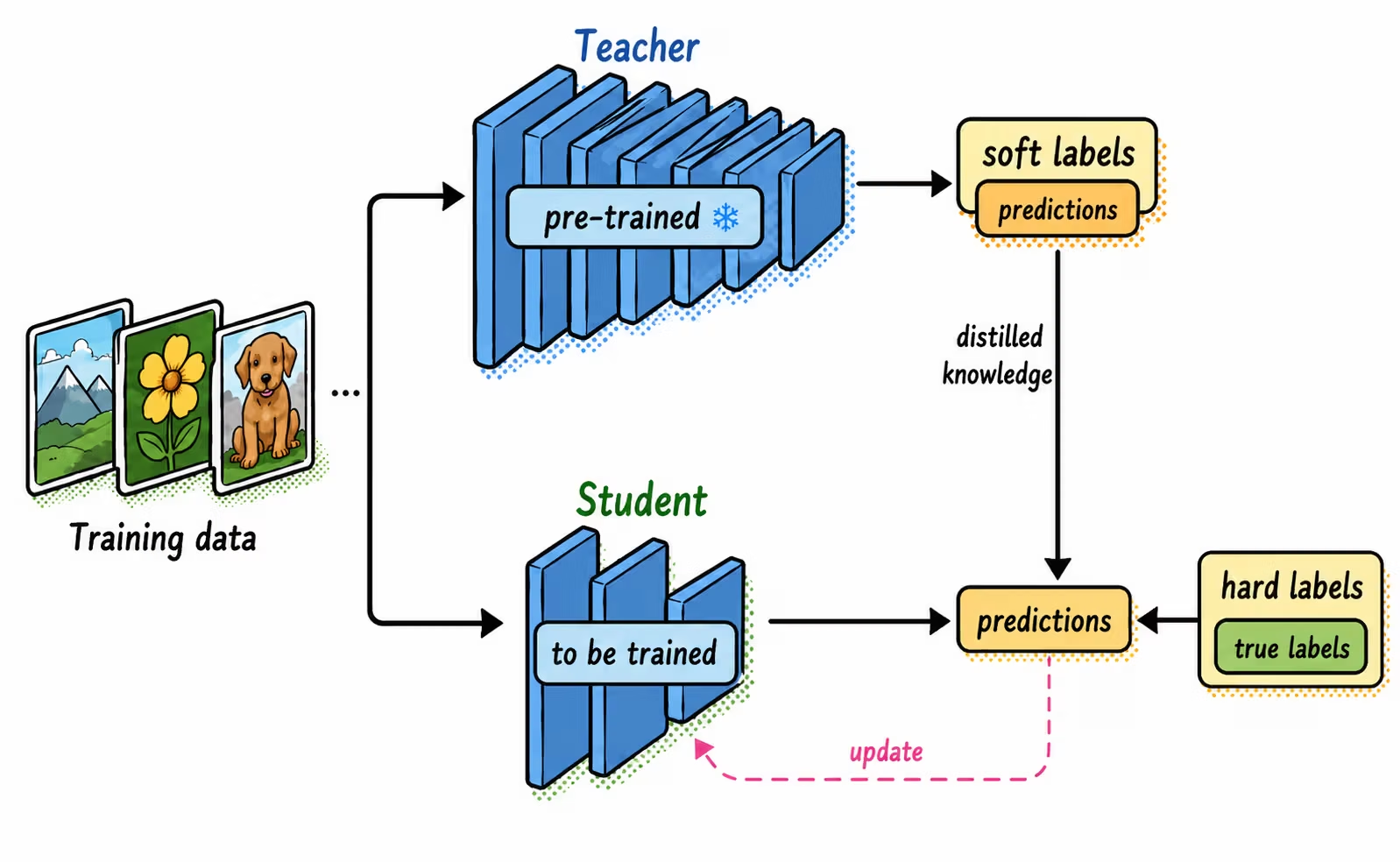
Knowledge distillation[hinton2015distilling] is a compression technique in which a large model, the teacher, supervises the training of a smaller model, the student.
The goal is to approximate the function the teacher has learned. If the transfer works, the student retains a significant part of its quality but with less memory, lower latency, and a lower inference cost. This approach is useful for producing lightweight models that can be deployed on mobile devices, edge devices, or services with heavy request volumes.
Hard labels and soft targets
In a conventional classification problem, a hard label indicates only the correct class. For an image of a cat, for example, the target vector might be:
for the classes cat, leopard, and dog. The teacher, on the other hand, can produce a distribution such as . These probabilities contain additional information: they show that, for the teacher, a cat is more similar to a leopard than to a dog. These relationships between classes are usually referred to as dark knowledge.
Soft targets are obtained by applying softmax to the logits (the model's unnormalized outputs) with a temperature :
When , the usual softmax is obtained. A higher temperature flattens the distribution and makes small probabilities visible, better exposing the similarities learned by the teacher.
Loss function
Let and be the smoothed distributions of the teacher and the student. A common formulation combines two objectives:
- The distillation loss forces the student to approximate the teacher's distribution. It can be expressed using Kullback–Leibler divergence or cross-entropy.
- The supervised loss compares the student's prediction with the true label .
The hyperparameter controls the relative weight of both terms. The factor compensates for the change in gradient scale produced by the temperature. It is not always essential to have human labels: unlabeled data or synthetic examples can also be used, training solely with the teacher's supervision.
Distillation in generative models
In an LLM, knowledge can be distilled at different levels:
- Logits: the student approximates the probability distribution over the next token. This approach requires being able to query the teacher's outputs and properly align vocabularies.
- Sequences: the teacher generates responses that become training data for the student. This is especially practical when only generated text is accessible.
- Intermediate representations: besides the output, hidden states or attention maps are aligned when the architectures allow it.
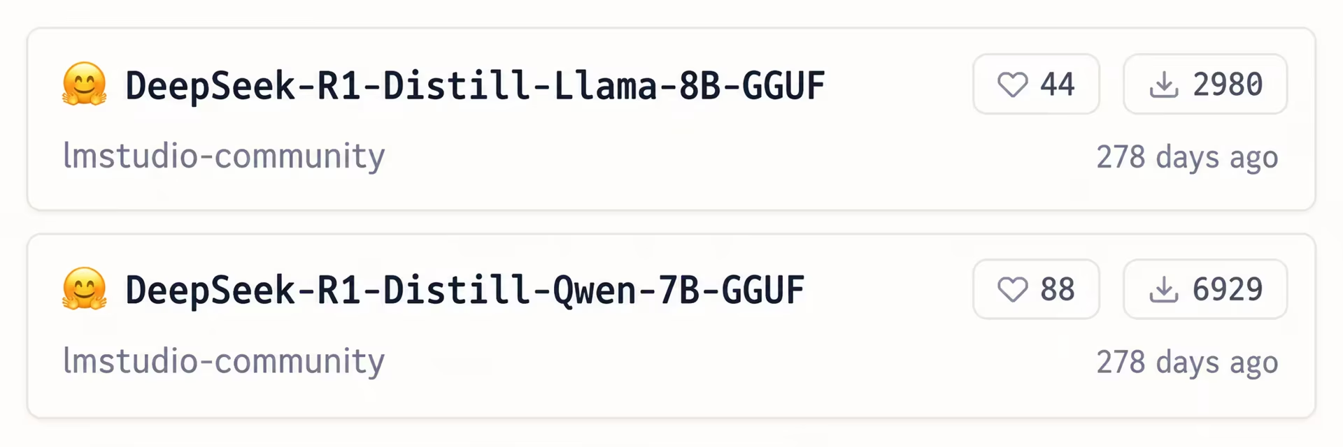
This is an example of sequence-level distillation: DeepSeek-R1 generates and filters solutions, and smaller models based on Qwen and Llama learn from those samples. They are not directly copying its logits.
Distillation has an upfront cost, the teacher must be run and the student must be trained, and it can transmit its errors or biases. Its usefulness depends on the accumulated savings during deployment offsetting that cost, and on the loss of quality being acceptable.
Quantization
Quantization is a technique for reducing computational and memory costs during inference by representing weights and activations with low-precision data types, such as 8-bit integers (int8) instead of the usual floating-point float32 or float16.
Reducing the number of bits means that the resulting model requires less storage in memory, consumes less energy, and operations such as matrix multiplication can be performed much faster.
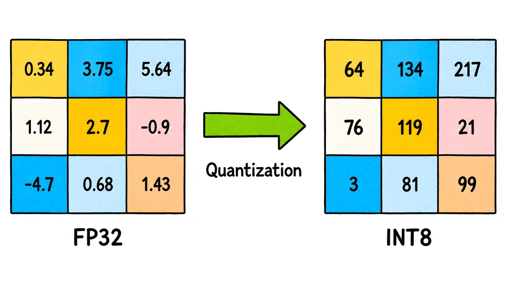
The most widely used standard method is uniform affine quantization, which maps real values onto a grid of integers through a linear transformation:
- Affine (asymmetric): allows the real value 0.0 to be aligned with an arbitrary integer (zero point), which avoids distortions when the data is not symmetrically centered around zero (as happens after ReLU-type activations).
- Uniform: the distance between two consecutive integers always represents the same fixed interval in the real-valued space (the scale factor s).
Mapping a real value to an integer is done as follows:
During inference, an approximation of is reconstructed:
Example - INT8 (range [0, 255])
Suppose the weights of a layer range between and :
- Scale (s):
- Zero point ():
- Quantize a value ():
- Reconstruct ():
The discrepancy between 1.2 and 1.1932 is the quantization error, generated by the rounding operation. To reduce this margin of error, the granularity at which and are computed is adjusted:
- Per tensor: all values in a layer share a single pair . It is very memory-efficient, but vulnerable to outliers.
- Per channel: each output channel has its own scale, balancing precision and computational cost.
- Per group: weights are divided into small blocks (e.g. 32 to 128 elements) with an independent scale, a technique fundamental to 4-bit LLMs (such as AWQ or GPTQ).
Which part of the model gets quantized?
- Weights only (weight-only): considerably reduces memory and is common in LLMs. Activations are kept at higher precision.
- Weights and activations: can speed up computation further, but activations are harder to quantize because they change with each input and can contain outliers.
- KV cache: in autoregressive models with long contexts, quantizing the cache reduces the memory that grows with the number of tokens processed.
The theoretical storage savings are easy to estimate. For example, for a 7B model:
| Weight format | Approximate memory |
|---|---|
float32 (32 bits) | 28 GB |
float16 / bfloat16 (16 bits) | 14 GB |
int8 (8 bits) | 7 GB |
| 4 bits | 3.5 GB |
PTQ and QAT
There are two main points at which quantization can be introduced:
- Post-Training Quantization (PTQ): an already trained model is quantized. It is fast and may only require a small calibration set to estimate scales. Methods such as GPTQ[frantar2022gptq] correct part of the error when quantizing LLMs weight by weight or block by block.
- Quantization-Aware Training (QAT): quantization operations are simulated during training so the model learns to tolerate the error[jacob2017quantization]. It tends to better preserve quality at aggressive precisions, but it requires retraining.
Quantizing always introduces a trade-off between size, speed, and quality. Layers do not all have the same sensitivity, and it is sometimes worth keeping some of them at higher precision. Moreover, a model that is four times smaller will not necessarily be four times faster: latency can be dominated by sequential generation, data transfer, or the lack of native support for the chosen format.
Low-Rank Adaptation (LoRA)
When training large generative models, adjusting all the parameters can be very costly, especially when the only goal is to adapt the model to a specific task.
In full fine-tuning, every weight matrix must have all of its parameters updated:
If , training requires up to parameters.
Low-Rank Adaptation (LoRA)[hu2021lora] is an efficient fine-tuning method, or PEFT (Parameter-Efficient Fine-Tuning), that seeks to reduce this burden using a technique called low-rank decomposition.
The central idea is to freeze the original weight matrix (some or all of the model's matrices) and, instead, decompose the update into the product of two smaller matrices:
where is a hyperparameter that scales the contribution of the low-rank update (often set relative to , hence the ratio ).
This way, instead of training values, only need to be trained. This significantly reduces the number of parameters that need to be adjusted, making the process more efficient.
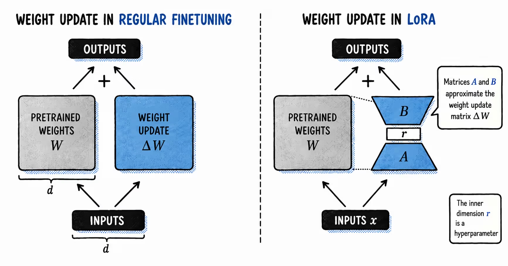
Example. Suppose we want to adapt a square weight matrix of size (a typical LLM layer), with parameters. Full fine-tuning of that matrix would update the M parameters. With , LoRA trains:
This represents approximately of that matrix's parameters.
There is a trade-off in choosing the rank. A rank that is too small may fail to capture the target task well. A very large rank improves capacity, but also increases cost and the risk of overfitting.
In general, there are two options:
- Merge the weights: compute the product and add it directly to the original matrix: . The model is saved with as a single standard file. This eliminates any latency or compute overhead at inference, but modularity is lost.
- Keep the adapter decoupled: only the file with the weights and is saved. At inference, the base model is loaded into memory and the input travels through two paths in parallel. On one hand, the base path, where is computed, and on the other, the LoRA path, where the adjustment is computed as . Both paths are then summed to obtain the final response.
To reduce memory usage during inference, LoRA can be combined with quantization. A popular combination is QLoRA[dettmers2023qlora]: it keeps the base model frozen and quantized, for example to 4 bits, and propagates the gradient through higher-precision LoRA adapters. This reduces both the memory of the base model and the memory associated with training.
Contributions
- Efficiency: allows models to be adapted without an exhaustive retraining, saving time and computational resources.
- Simplicity: for each task, only an adapter needs to be saved instead of a full copy of the model.
How to choose a technique
| Main goal | Technique | What is reduced | Main trade-off |
|---|---|---|---|
| Create a small model to serve many times | Distillation | Parameters and inference compute | Training a student and accepting some loss of quality |
| Adapt a model on a tight budget | LoRA | Trainable parameters and optimizer states | The base model is still required |
| Load or run a model with less memory | Quantization | Bits per weight and, optionally, per activation | Numerical error and dependence on hardware |
| Adapt a model that barely fits in memory | QLoRA | Base model memory and fine-tuning memory | More complex training and quantization operations |
These techniques can be chained together. For example, one can distill a large model, adapt the student with LoRA, and quantize the result for deployment.