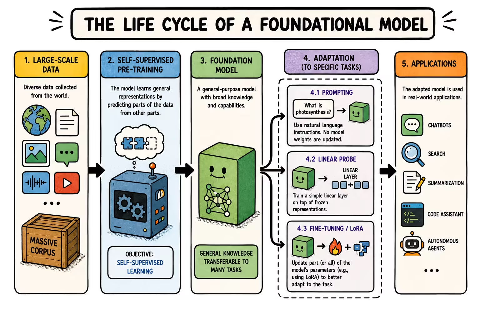
Foundation Models
In the previous chapter we saw how a Transformer can be trained autoregressively. Given a sequence of tokens, the model learns to predict the next one. This is a form of self-supervised learning. In this type of paradigm, if we train a sufficiently expressive model with a general task and a broad collection of data, the representations it learns can be reused to solve problems that were not explicitly defined during training.
This shift in perspective, from training a model for each task to pretraining a base that can adapt to many tasks, is the origin of foundation models.
Self-supervised learning
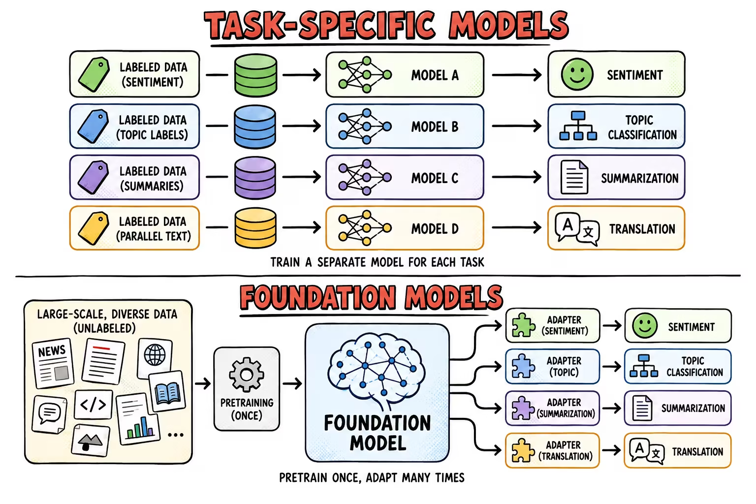
Imagine we want to classify the opinion of a review as positive or negative. Traditionally, what was done was to build a dataset of pairs , where is the text and is its label, and from there train a model to approximate .
Now imagine that instead of classifying positive/negative we want to assign one to five stars → we would have to re-label all the data. Every problem would need new labels and, usually, a new training process.
This strategy works but:
- Labels are expensive: they require annotators and consistent criteria.
- Knowledge stays fragmented: each model only learns what it needs to solve its own task.
- Reuse is limited: a change in the categories or the domain can force us to label data and train again.
The problem is not supervised learning itself. Human labels are still essential. The problem is using large amounts of task-specific supervision to learn from scratch everything that each task shares with the others.
Self-supervised learning has a history that predates modern training at scale, but the availability of large collections of text, images, audio, and video accelerated its adoption. This does not mean training happens without labels, but rather that the targets are obtained from the data itself instead of being manually annotated.
The transition did not happen overnight, nor did it eliminate supervised learning. It was an accumulation of ideas:
- Task-specific models: one architecture and one labeled dataset for each task.
- Transfer learning: reusing features learned on a large problem.
- Self-supervised pretraining: learning most of the parameters with data that has no manual annotations.
- Pretraining at scale: jointly increasing the diversity of the data, the capacity of the model, and the compute.
- General-purpose adaptation: using fine-tuning, prompting, or in-context learning to address many tasks from the same base.
In natural language processing, models like BERT[devlin2018bert] showed that an encoder pretrained on unlabeled text could be adapted with few modifications to numerous tasks. On the other hand, the GPT family showed that scaling autoregressive decoders made it possible to reuse the same model through examples or instructions written directly in the context.
What is a foundation model
The term foundation model was popularized to describe models trained on broad, large-scale data that can adapt to a wide range of downstream tasks[bommasani2021foundation].
The word foundational does not imply that the model is finished or universal. It simply describes an incomplete base on which later systems are built.
We can think of four ingredients:
- Broad data: covering many concepts, contexts, or modalities.
- General objective: not tied to a single label or application.
- Scalable architecture: can absorb more data and capacity without being redesigned for each task.
- Adaptability: its representations or predictions can be reused in new problems.
LLMs are, therefore, one type of foundation model, but there are also foundation models for vision, audio, video, or multimodal systems.
Relevance of the Transformer
Self-supervised learning predates the Transformer and does not require this architecture. However, the Transformer brought together several properties especially suited to pretraining at scale:
- Parallelization during training.
- Long-range dependencies via self-attention.
- It can adapt to different modalities: text tokens, image patches, audio fragments, multimodal sequences...
- The same structure scales by increasing layers, dimensionality, data, and compute.
Encoders and decoders
The original Transformer[vaswani2017attention] used both: the encoder to build a contextual representation of the input sequence, and the decoder to generate the output sequence. Modern variants can keep both components or use only one of them.
Encoder-only
In an encoder, each token can normally attend to all the other tokens in the input. The representation of a word can use both the preceding and the following words:
This bidirectional visibility produces contextual representations that are very useful for:
- classification and regression
- information extraction
- semantic search
- segmentation or detection in images
- building embeddings for other networks
BERT[devlin2018bert] is a clear example of this.
Decoder-only
In a causal decoder, each position can only use itself and the previous positions:
This restriction allows the output to be interpreted as a distribution over the next token and to generate a sequence step by step. It is the natural configuration for language models.
It is worth noting that a decoder is not limited to "writing text" — its internal states also contain useful representations. However, its training and usage setup is especially aligned with open-ended generation.
Encoder-decoder
The encoder processes a complete input and the decoder generates an output conditioned on it:
This separation is natural when the input and the output play different roles, as in translation, summarization, image captioning, or conversion between modalities.
Other compositions
Foundation models do not always fit into those three classic configurations. For example, CLIP[radford2021clip] uses a dual encoder to process two modalities separately and project their representations into a shared space, in this case images and text. Another example is JEPA, where a context encoder + target encoder + predictor architecture can be used to predict a target representation.
Pre-training tasks
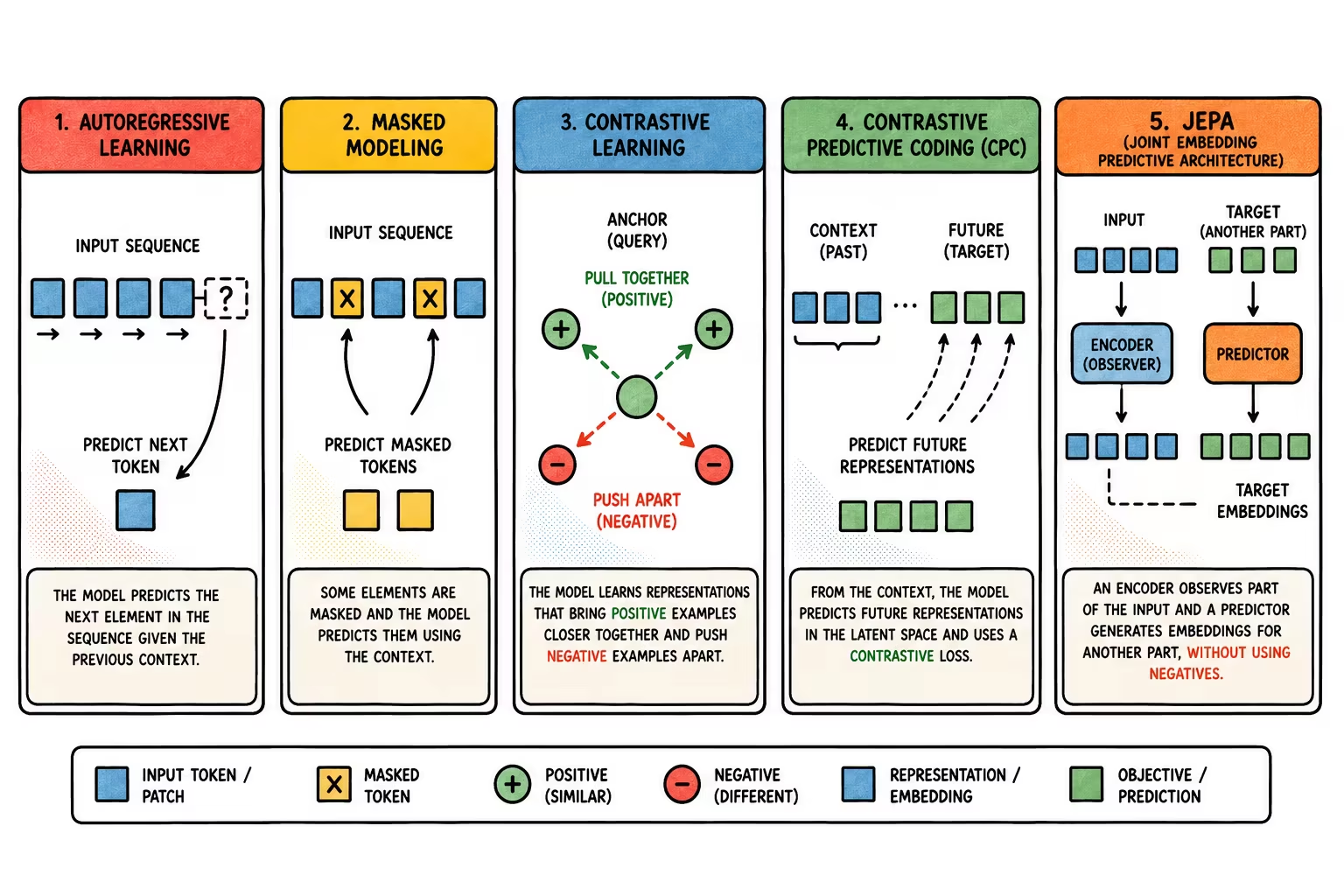
So far we have talked about self-supervised learning in general terms, but this only describes where the supervision comes from. However, there are different paradigms. To compare them it is useful to ask what information the model receives and what it must predict.
Autoregressive learning
As we saw in the previous chapter, an autoregressive model factorizes the joint probability of a sequence:
Its usual loss function is the cross-entropy between the actual next element and the predicted distribution:
Each position acts as a new target, and the objective coincides with the generation procedure, which makes the causal decoder a direct generative model.
Masked modeling
Another possibility is to hide or corrupt part of the input and ask the model to reconstruct it. If is the set of masked positions:
In masked language modeling (MLM), the encoder observes the context on both sides of the gap:
"The player [MASK] their cards" → "showed".
BERT uses this objective to pretrain an encoder that can later be adapted to supervised tasks.
The same idea can be carried over to other modalities. In images, Masked Autoencoders (MAE) are commonly used, which consist of removing a high proportion of patches, processing only the visible ones with an encoder, and using a decoder to reconstruct the missing pixels[he2021mae]. Once pretraining is finished, the decoder is discarded and the encoder is kept as the foundation model.
Contrastive learning
Instead of reconstructing the data, the model can be taught which samples should have similar representations.
We usually start from a sample , from which two related views and are generated. In an image these might be two crops with color changes; in a multimodal system they might be a photograph and its caption. They are then passed through an encoder that turns each view into an embedding:
A contrastive loss pulls the positive pair together and pushes it apart from representations corresponding to other samples. A common form is InfoNCE[oord2018cpc]:
where is a temperature and is usually cosine similarity.
The encoder is taught which changes it should ignore and which relationships it should preserve. SimCLR[chen2020simclr], for example, treats two transformations of the same image as positive. CLIP aligns corresponding images and texts to build a space shared across modalities.
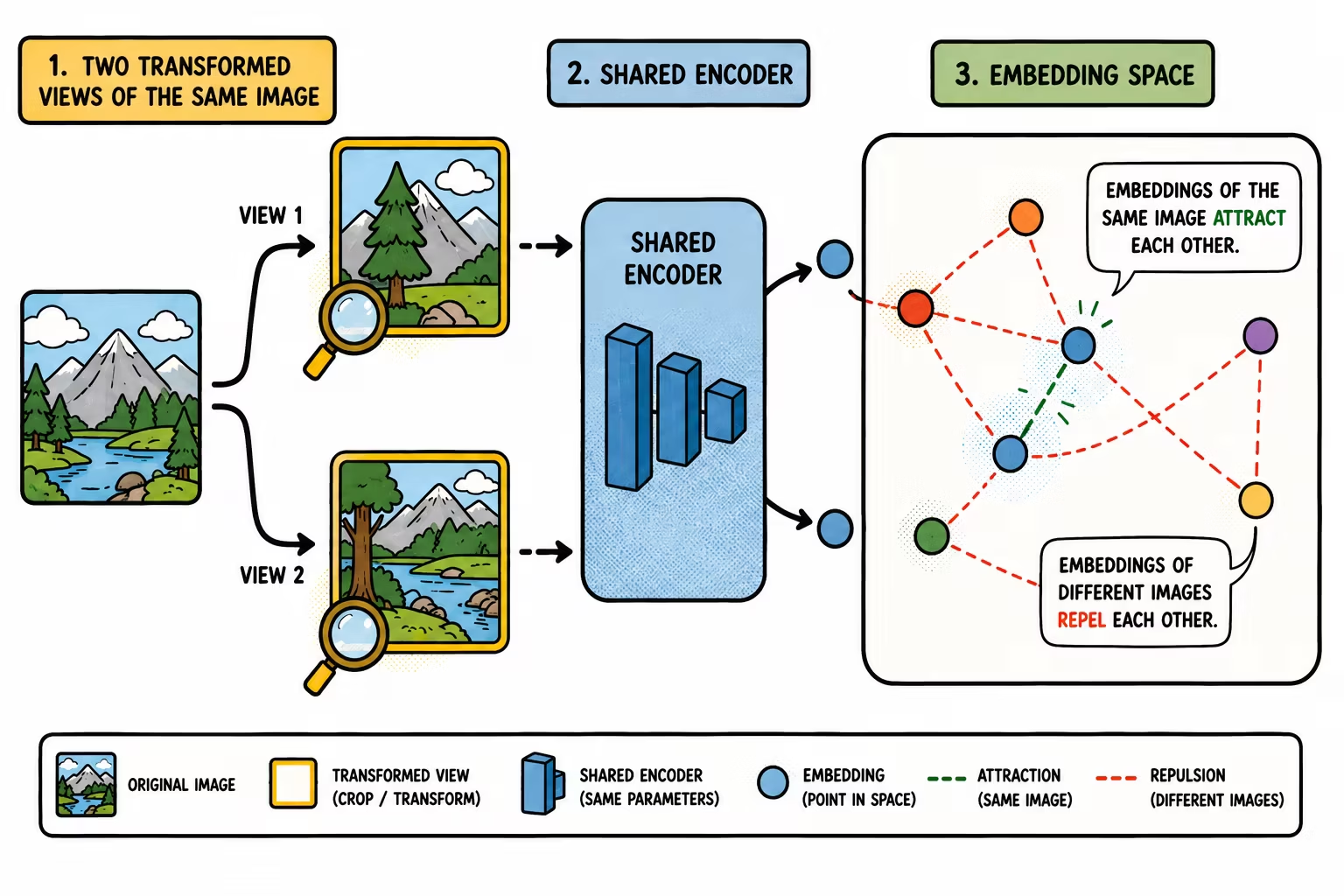
The choice of views is crucial. If two transformations are considered equivalent, the model will learn to be invariant to their differences. A poorly chosen transformation can eliminate precisely the semantic property that makes two images have something in common.
Contrastive Predictive Coding (CPC)
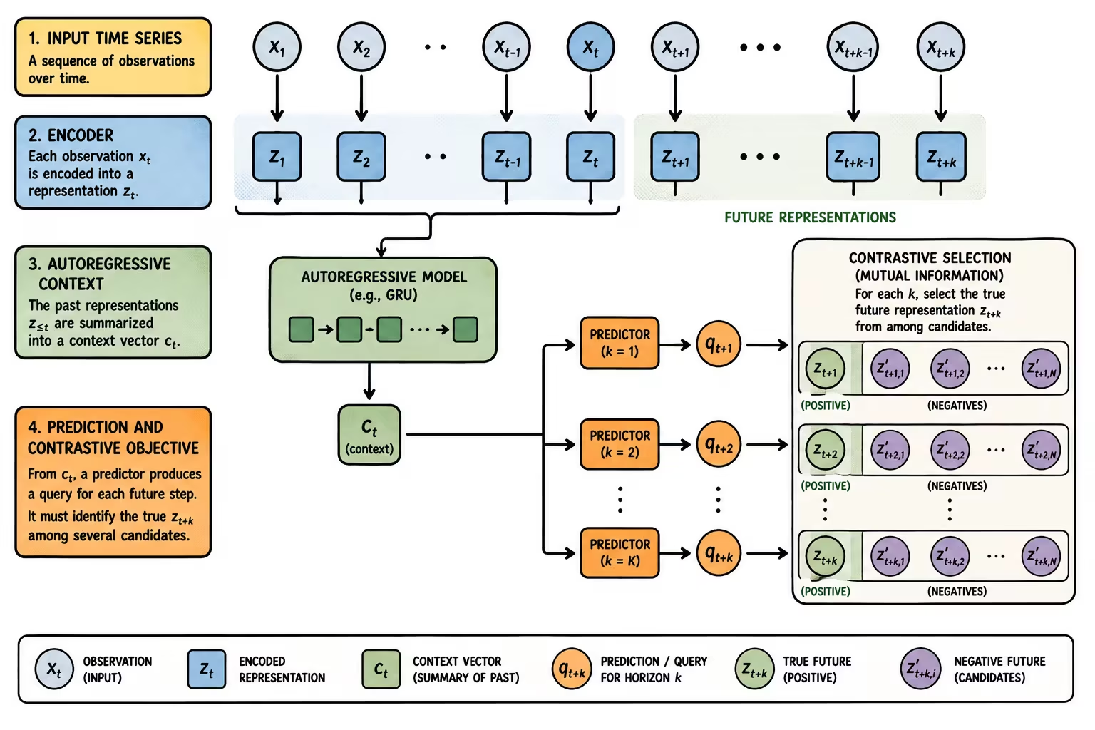
CPC[oord2018cpc] combines temporal prediction, latent representations, and contrastive learning.
First, an encoder transforms each observation into a representation . Then, an autoregressive model summarizes the past into a context vector :
From , the model must identify the correct future representation among several negative samples. It does not try to reconstruct anything, but instead retains the information that allows it to distinguish the real future from plausible alternatives.
CPC occupies an interesting position among several families:
- it is autoregressive because it summarizes the past to anticipate the future,
- it is contrastive because it distinguishes positive targets from negative ones,
- it is predictive in latent space because the target is a representation, not the full observation.
From observations to representations
Reconstructing high-dimensional data can be unnecessarily difficult. To complete an image, a model might have to decide the exact texture of a wall or the position of every leaf on a tree. These are details that are hard to predict and perhaps irrelevant if what we later want is to recognize objects or understand a scene.
We can express the difference schematically:
The second option allows the target to omit unpredictable details and retain more abstract properties. This is the main motivation behind Joint-Embedding Predictive Architectures.
JEPA
Joint-Embedding Predictive Architectures (JEPA)[lecun2022path] were put forward by Yann LeCun as part of a broader proposal for building machines capable of learning internal models of the world. We will first study JEPA as a pretraining method, and later connect these representations with agents, planning, and world models.
JEPA is not a specific network, but a family of architectures and objectives. We usually talk about three components:
- A Context Encoder transforms the observed part into a latent representation .
- A Target Encoder transforms another related view into the target representation .
- A Predictor uses and some information about the relationship between the two views to estimate .
Schematically:
where describes which target is to be predicted, measures the distance between representations, and indicates that the gradient does not update the target encoder.
During pretraining, both encoders observe related views of the same data. The Target Encoder and the Predictor are auxiliary training components and can be discarded afterward. What is worth keeping as the foundation model is the Context Encoder.
On the other hand, in some formulations it is considered that the same situation could have several compatible futures: the Predictor then receives an additional latent variable from which it selects among different possible predictions. This is not universal to all JEPA (the example we will see next, I-JEPA, is deterministic), but when it is present it can be worth keeping the Predictor as well, to anticipate the evolution of the latent state. This issue is especially important in video and robotics, where the future is not fully determined by the current observation.
Let's look at a more concrete example.
I-JEPA: learning from regions of an image
I-JEPA[assran2023ijepa] (Image-based JEPA) brings this principle to visual learning. From the same image it builds:
- a context block, made up of visible, spatially distributed patches,
- several target blocks, corresponding to regions that the context encoder cannot observe,
- a positional encoding for each target block.
The context encoder processes only the visible patches. The target encoder computes the representations of the target blocks, and the predictor tries to recover them from the context and their position. It does not reconstruct the original pixels, but instead predicts the embeddings that the target encoder would have produced for those regions.
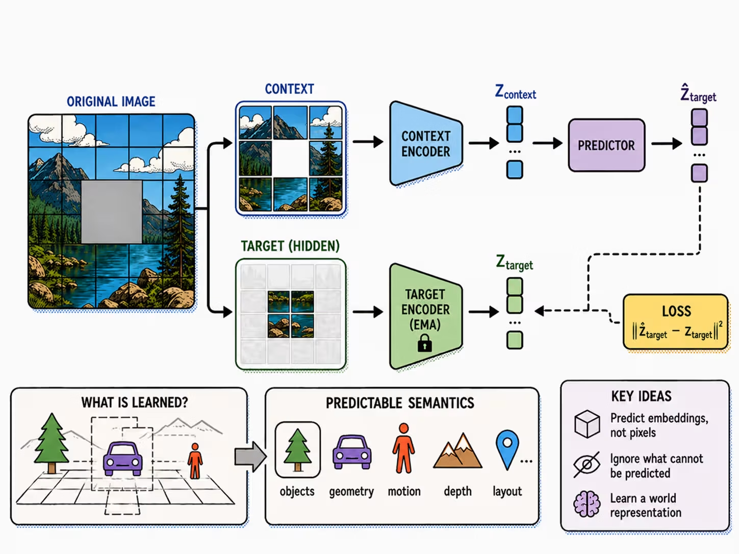
The masking pattern matters. If the targets are too small, the model can solve the task using local textures; if the context contains little information, the target becomes impossible to anticipate. I-JEPA uses relatively large target blocks to favor semantic properties, and a distributed context that provides enough information about the scene.
V-JEPA: From images to video
In V-JEPA[bardes2024vjepa], the related views come from a video and masking extends across space and time. The model predicts the representations of hidden spatio-temporal regions from the visible video. This forces the encoder to capture both appearance and motion, without reconstructing pixels, using text, relying on negative examples, or starting from a pretrained image encoder.
The collapse problem
During training there exists a useless solution that would nonetheless minimize the error: having every input produce exactly the same embedding. In that case, the predictor would always be correct without learning anything about the data:
This is called complete collapse, but there is a subtler variant: the embeddings can be different and yet concentrate almost all of their variability in a few dimensions. In this dimensional collapse, the model wastes much of the latent space and produces poor representations for downstream tasks.
Joint embedding methods need to prevent these problems. Contrastive approaches do so by pushing negative examples apart. Other methods use normalization, terms that enforce variance and decorrelation, a slowly updated target encoder, or stop-gradient.
I-JEPA uses two related mechanisms:
- The gradient of the loss updates the context encoder and the predictor, but not the target encoder.
- The parameters of the target encoder follow an exponential moving average of the context encoder's parameters. The target changes slowly and provides a more stable reference.
These mechanisms work, but they introduce design decisions: the speed of the moving average, asymmetry between branches, the predictor, and the masking strategy. Much of the research on joint embeddings has focused on finding recipes that avoid collapse without degrading the quality of the representations. This is precisely the problem LeJEPA tries to address.
LeJEPA
LeJEPA[balestriero2025lejepa] (Latent-Euclidean JEPA) is a formulation proposed by Randall Balestriero and Yann LeCun that attempts to replace those heuristic recipes with an explicit criterion for how the latent space should be organized.
LeJEPA starts from two minimal requirements:
- Predictability: representations of related views should be able to predict one another.
- Non-degeneracy: embeddings must occupy the latent space in a way that is suitable for downstream tasks.
The first requirement provides invariance: two related views of the same sample should preserve the same semantic information. On its own, however, it allows all views and all samples to be represented by the same single point. The second requirement must rule out both complete collapse and dimensional collapse.
The authors analyze which distribution of embeddings would, under the assumptions of their theoretical framework, reduce the expected risk across a broad family of downstream tasks. Their result proposes an isotropic Gaussian as the objective.
This geometry prevents all points from coinciding, some dimensions from staying constant, or information from concentrating in a small subspace. Requiring only zero mean and identity covariance does not, however, control the whole shape of the distribution, since very different distributions can share those two first properties.
SIGReg
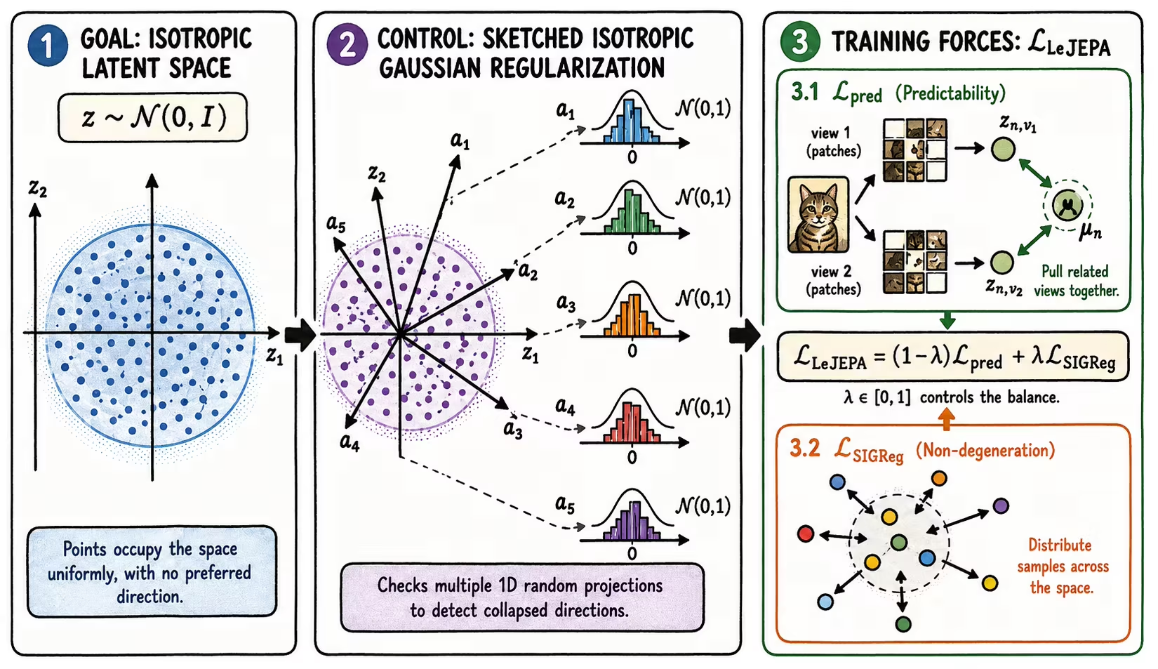
Checking and directly regularizing a distribution with hundreds or thousands of dimensions would be very costly. Sketched Isotropic Gaussian Regularization (SIGReg) reduces the problem to multiple one-dimensional checks.
For each random unit direction , the embedding is projected:
If follows an isotropic Gaussian, any projection must follow a one-dimensional Gaussian . SIGReg samples several directions, compares the empirical distribution of those projections with the target Gaussian, and resamples directions during training. This way it can detect a collapsed direction without explicitly constructing or comparing high-dimensional densities.
The proposed implementation uses a test based on characteristic functions, related to the Epps–Pulley statistic. This choice provides bounded gradients and a cost that grows linearly with the number of samples, which makes it possible to apply the regularization to large embeddings and models.
The LeJEPA loss
Let be the representation of view of sample . LeJEPA builds a center from the global views. For a given sample , the following expression is the per-sample predictive loss:
This simplified equation pulls together the views of the same sample. The full formulation averages that term over the samples in the batch and applies SIGReg separately to each view, using the embeddings from the whole batch:[balestriero2025lejepa-formulation]
The two terms exert complementary forces:
- The average of pulls together the views of each sample and removes irrelevant variation.
- SIGReg organizes, for each view, the representations of the samples in the batch and prevents them from ending up at the same point or subspace.
The only hyperparameter specific to the combination is , which regulates the balance between predictability and diversity.
What it simplifies
By preventing collapse through an explicit objective on the distribution, LeJEPA's recommended recipe can use the same encoder for the different views and dispense with several usual components, such as:
- negative examples and large sample queues
- teacher-student networks and their moving-average schedule
- stop-gradient
- a predictor used solely to avoid collapse
- prototypes or special output dimensions
Another practical property is that the training loss reported by the authors correlates with the quality of the representations as measured by linear probing. In many self-supervised methods a lower loss does not necessarily imply a better encoder, which forces supervised evaluations to be run during development. If this relationship holds in new domains, it would make it possible to select models without relying on labels.
World models
We began the JEPA section by noting that these architectures were put forward as part of a proposal for building machines capable of learning internal models of the world. This idea connects directly with world models.
A world model is a learned model of the dynamics of an environment: given a representation of its current state, it predicts how it may evolve. If there is an agent acting on the environment, the prediction must also depend on the action it takes.
In simplified form, it contains two pieces:
- A state encoder transforms the observation (or the recent history) into a latent state .
- A transition model predicts the next state from the current one and the action :
Depending on the application, the world model can also predict rewards, events, or a distribution over future states instead of a single state.
What JEPA contributes
A world model needs a state space that retains what determines the evolution of the environment. Foundation models obtained via JEPA provide precisely a starting point for building it.
However, a pretrained encoder is not yet a world model. Learning dynamics requires temporally ordered data and a transition predictor. Actions are needed when we want a model conditioned on an agent's intervention and want to use it for control.
This relationship can be summarized as follows:
Simulation and planning
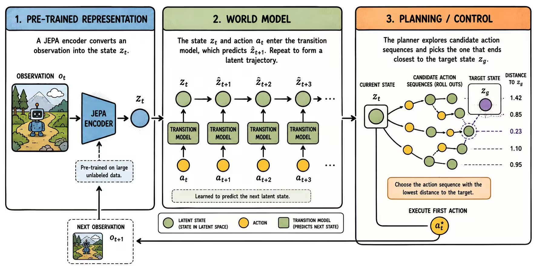
Once learned, the world model can be used as a latent simulator. If we have a target state , we can:
- Encode the current observation as and the goal as .
- Propose several action sequences.
- Roll out their consequences in latent space via .
- Measure which predicted final state ends up closest to .
- Execute the best action and plan again with the new observation.
The system only simulates the latent variables needed to compare their consequences. This can be much more efficient than generating full observations, and it avoids spending capacity on details that are irrelevant to the decision.
In a robotic arm, for example, can encode the position of a cup and of the arm, the opening of the gripper, spatial relationships, and possible contacts. The world model allows the gripper's movements to be rehearsed before being executed physically. It can also be used as a simulator to train policies, generate hypothetical trajectories, or assess whether an action could cause a collision.
V-JEPA 2[assran2025vjepa2] is an example of this transition. After visual pretraining, its V-JEPA 2-AC variant incorporates robotic trajectories with actions to learn the dynamics . The predictor is then used to plan reaching, grasping, and placing tasks from a visual goal.
Comparison
| Paradigm | What is hidden or related | Target | Target space | How it avoids a trivial solution | Architecture |
|---|---|---|---|---|---|
| Autoregressive | The future | Next element | Data | Must explain the actual token | Decoder |
| Masked modeling | Parts of the input | Hidden tokens or pixels | Observation space | Must reconstruct the actual content | Encoder or encoder-decoder |
| Contrastive | Two related views | Correct pair | Latent | Negatives or batch distribution | Encoder |
| CPC | Future of the sequence | Correct future representation | Latent | Contrastive negatives | Predictive encoder |
| JEPA | Missing or future region | Target representation | Latent | Teacher, stop-gradient, or other mechanisms | Encoder |
| LeJEPA | Context and target views | Representation + regularized geometry | Latent | SIGReg | Encoder |
*Note that this table does not describe fully mutually exclusive categories.
Downstream tasks
The result of self-supervised learning is not an assistant, a classifier, or a search system. It is a base on which to build a useful system. For that, there are different options:
Linear probing
The encoder is frozen and a linear layer is trained on its representations with a labeled dataset. It is a common way to measure how much accessible information the embedding contains without modifying the pretrained model.
Fine-tuning
Training continues on all or part of the parameters using examples from the final task. It usually provides more adaptation capacity, but requires storing and updating a large model.
Efficient adaptation
Methods like LoRA[hu2021lora] update a reduced number of parameters and keep most of the base model frozen. We will cover them in the next chapter.
Prompting and in-context learning
In a generative model, the input itself can describe the task and include examples. The model adapts its behavior through the context without its parameters changing:
Classify the review as positive or negative. Review: "The story is slow, but the characters are wonderful."
This mechanism reduces the need to create a different output head for each task: many applications can be expressed through a common text or token interface.
Post-training and alignment
LLMs pretrained solely to predict the next token do not automatically behave like assistants. After pretraining, instruction data, demonstrations, and preferences are used to improve their ability to follow requests.
This is where techniques such as the following come in:
- Supervised fine-tuning (SFT) on instruction-response pairs.
- RLHF[ouyang2022instructgpt], which uses human preferences to train a reward signal and optimize the model.
- Direct preference optimization methods, such as DPO[rafailov2023dpo].
These techniques belong to post-training. They are not self-supervised paradigms comparable to MLM, CPC, or JEPA, because they use additional supervision to modify the behavior of an already pretrained base.