Transformers

Background

To understand the origin of Transformers we need to review some concepts we haven't covered yet.

From words to vectors

So far we have covered architectures mainly oriented toward images, which makes their processing easier because they already come in numerical format (images are matrices of pixels), but Transformers deal with text. Neural networks don't understand words, so the text has to be transformed into a numerical representation.

One-Hot Encoding

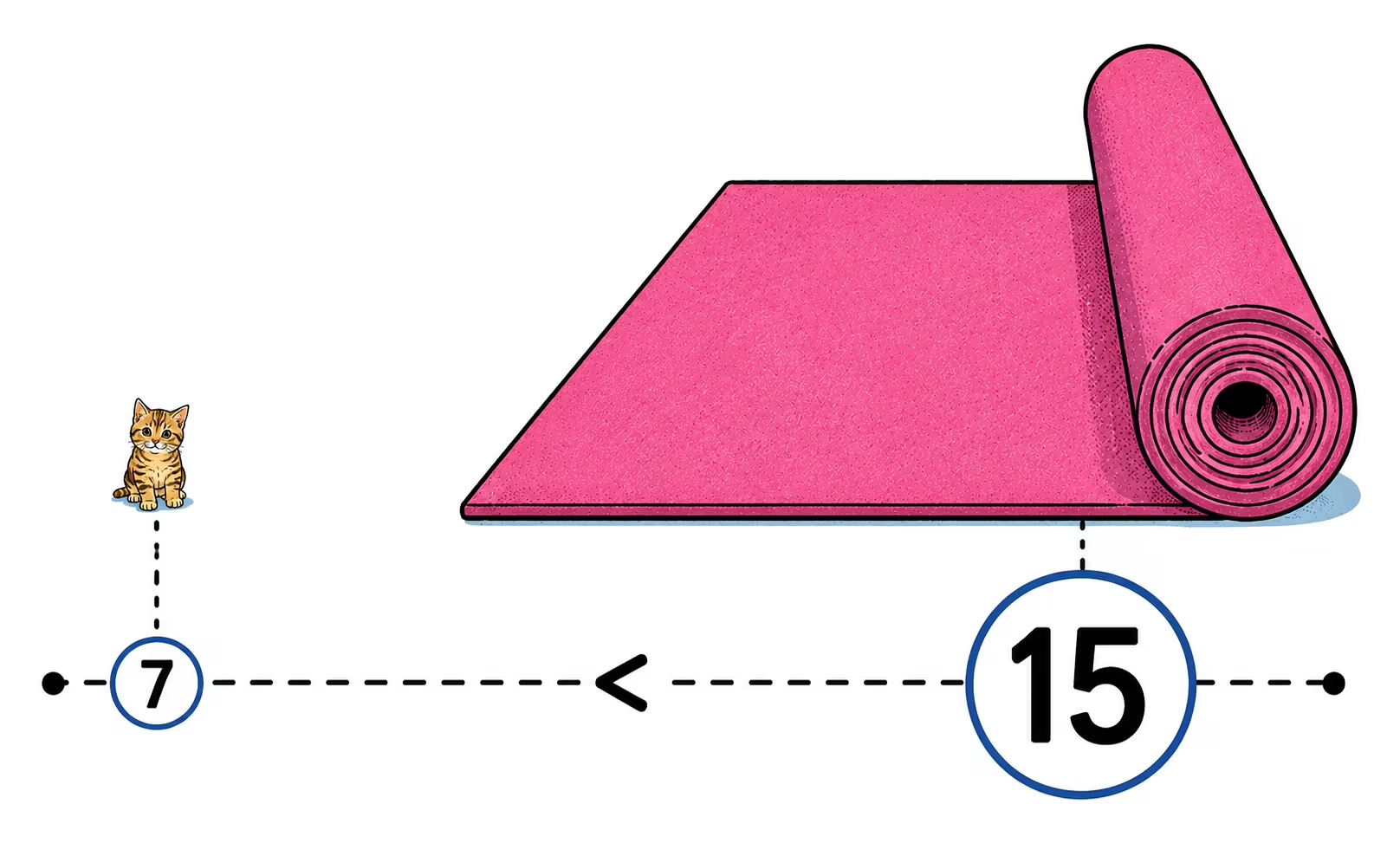
The most basic approach would be to associate each word with a number. For example, we could represent the sentence "The cat sat on the mat" as a vector "[25, 7, 4, 8, 27, 15]".

❗ Problem → If we fed those identifiers directly in as numeric values, we would be telling the model that words with a larger associated number carry more importance.

💡 Instead, each word could be associated with a vector with as many positions as there are words in the vocabulary of the problem at hand. To represent a word, a 1 would be marked in the position that corresponds to it and 0 in the rest. For example, if the vocabulary only had 3 words we would have something like the following:

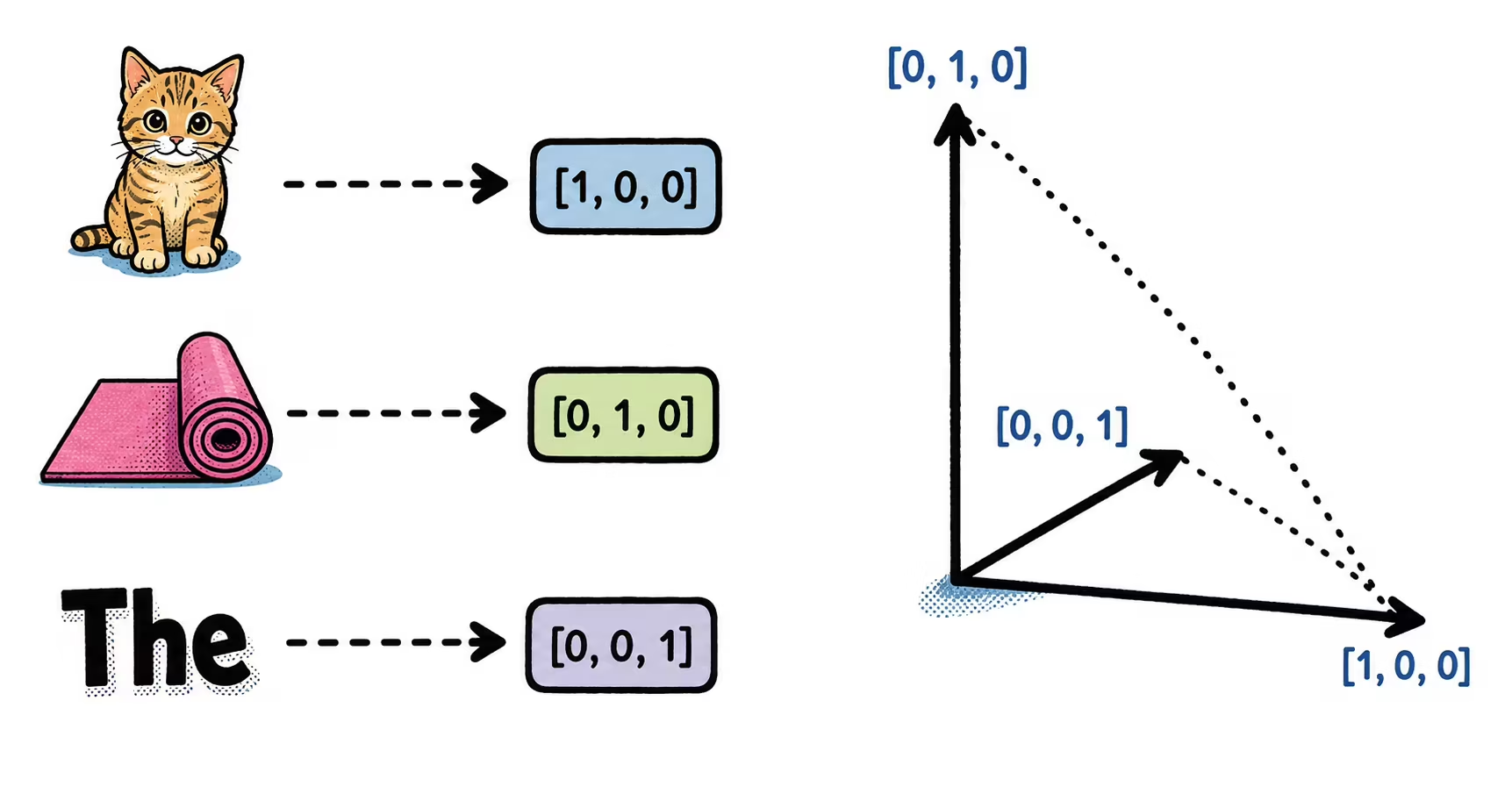
With this representation the distance between words is preserved! This happens regardless of the number of words (dimensionality) in the vocabulary.

❗ However:

• Unnecessary storage: a 10-word sentence with a 400-term vocabulary becomes a 10×400 matrix where most values are 0.
• All words are equidistant: this solves the previous problem, but words like "cat" and "box" should actually be closer together than "cat" and "sky".

Embeddings

Related to this last point, we as humans understand that some words are semantically more related to each other than others. "car", "mechanics" and "wheel" are conceptually closer to each other than "cloud" or "volcano".

For example, how would you mentally sort the images on the left?

One option could be by color and type of car → It would end up looking something like the image on the right.

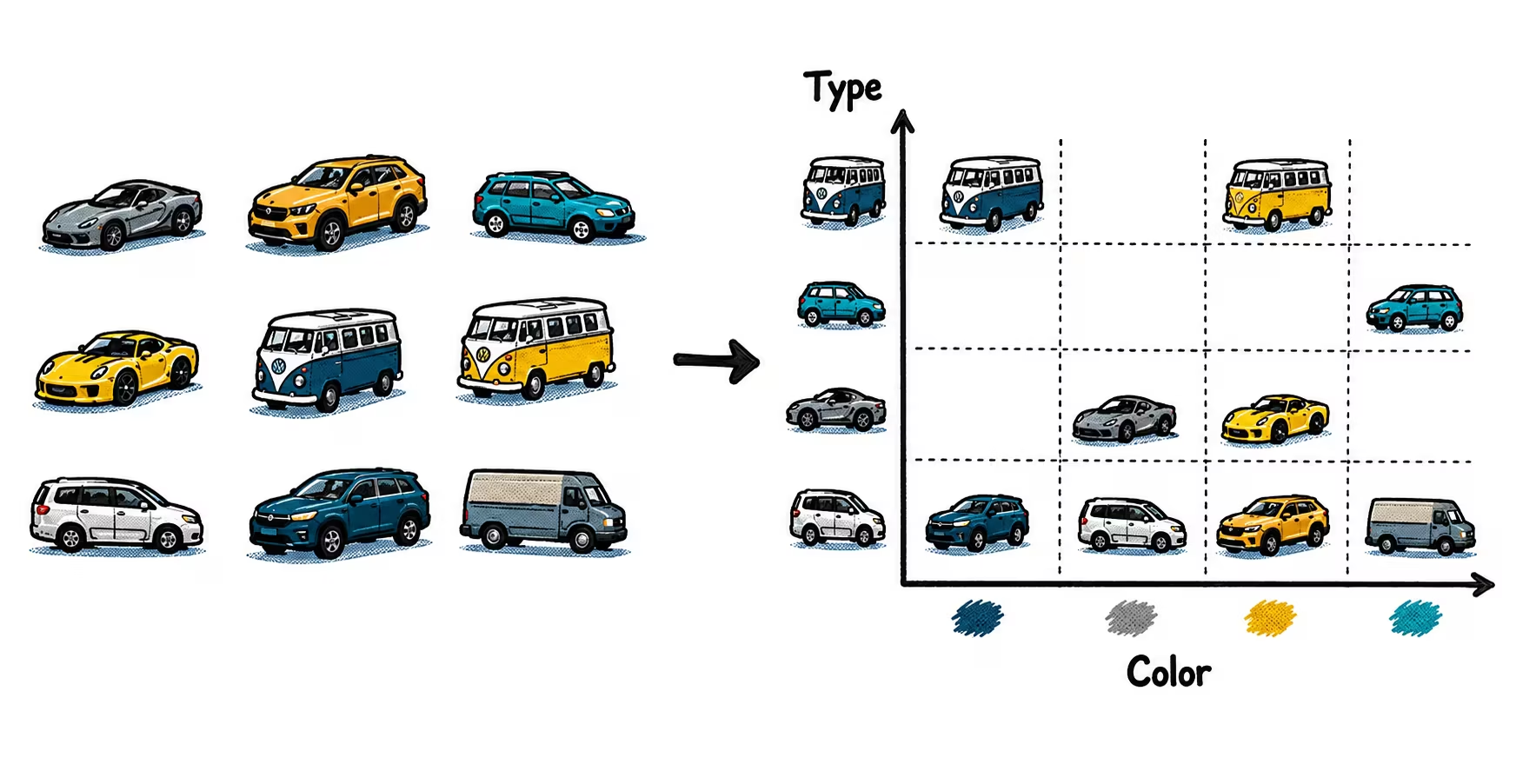
Internally we follow a process of compressing and ordering data.

To begin with, each image has thousands of pixels, which our brain processes and orders until it obtains a much more compact representation. In other words, it has performed a dimensionality reduction, in this case down to two dimensions. This is precisely one of the operating principles of neural networks: compressing and ordering data until obtaining an internal representation (latent space or embedding) useful for downstream tasks.

This doesn't happen only with images; any data that can be converted into a numerical representation can be subject to this same process. We already saw that text can be converted into a numerical representation, whose dimensionality is very large, so it can be modeled to reduce/compress it.

At first, the embedding layer has no knowledge of how to organize the data, but, as it is trained, it learns representations suited to solving the task. For example, when analyzing whether a movie review is positive or negative, words like "happy", "satisfying" or "like" will tend to end up close together.

Tokens

In practice, text is not split into words but into numeric units we call tokens.

Tokens are indices within a vocabulary: the number 1437 doesn't mean anything by itself, it's simply a position that points to an embedding. The embeddings for each token are initialized randomly and, as the model sees words during training, it adjusts the values of each vector to obtain the best representation of each one.

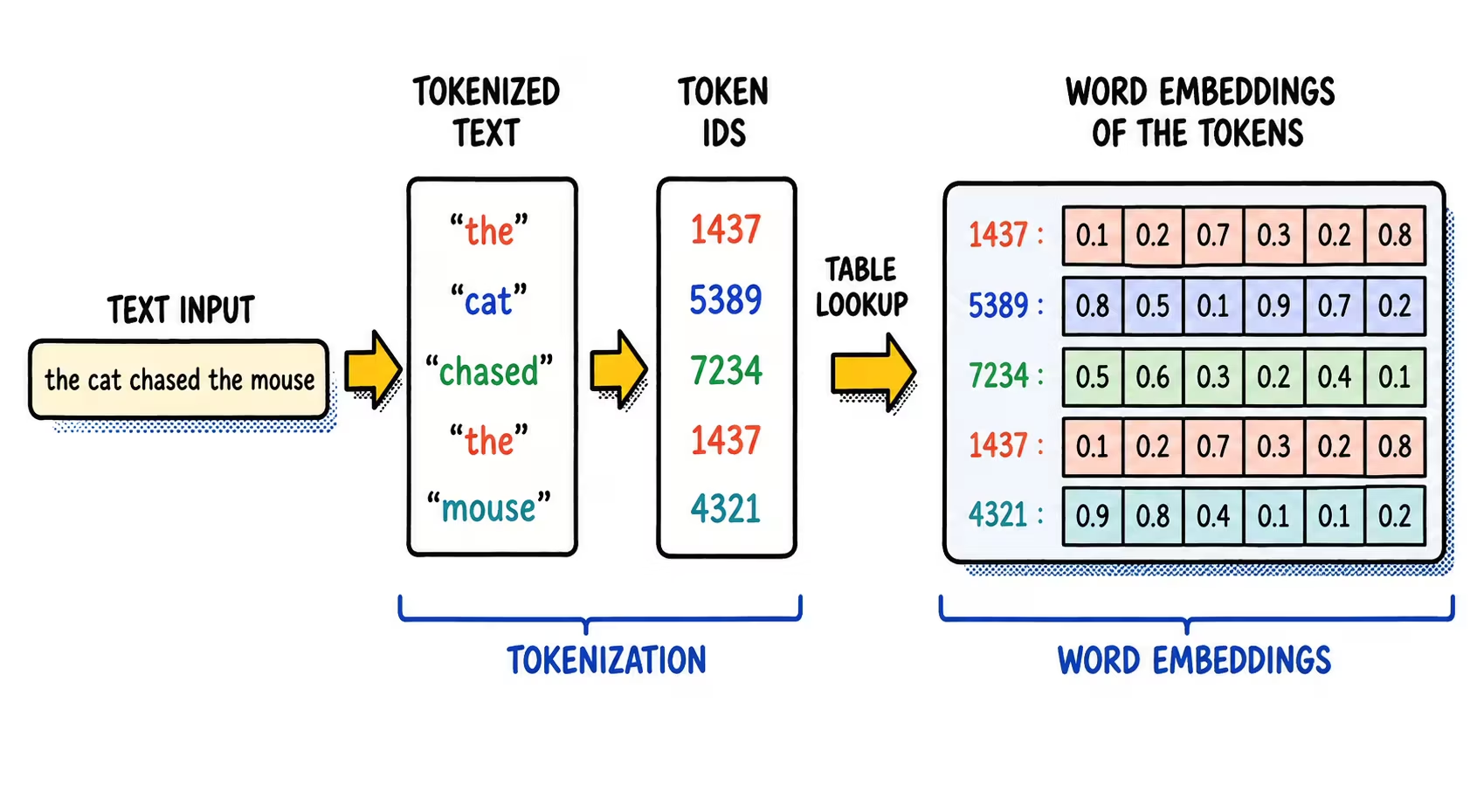
There are different ways to tokenize text, so each model usually has its own tokenizer (typically based on algorithms such as Byte Pair Encoding (BPE), SentencePiece (Unigram) or WordPiece), understood as a component that converts text into tokens.

Recurrent networks and Vanishing Gradient

Going back to the modeling side, many machine learning tasks were initially solved with simple neural architectures. Over time, architectures evolved to adapt to the nature of the data:

• Images → Convolutional Neural Networks (CNNs)
• Data organized as graphs → Graph Neural Networks (GNNs)
• Sequential data, such as text or time series → Recurrent Neural Networks (RNNs)

In sequential data, order matters. When processing a word, for example, it's necessary to take the previous words into account because they provide the context that allows it to be interpreted. Recurrent networks are precisely useful for this because they incorporate connections that reuse the information processed in previous steps (unlike a multilayer network, whose connections only move forward toward the output).

In an RNN, the first word is processed and the resulting state is fed into the processing of the next one. The process repeats until the whole sequence has been traversed. Thus, the state of the network at each step depends both on the current input and on the previous states, hence the name recurrent network.

The main problem with RNNs is that, when sequences are very long, the influence of the earliest elements on the last ones can become smaller and smaller. The network ends up "forgetting" information from the start of the sequence, a problem related to what is known as the vanishing gradient.

LSTM and GRU architectures mitigate this problem through mechanisms that control which information is kept, updated or forgotten. Even so, each state depends on the previous one, which is a problem because it limits the handling of very distant dependencies and also makes parallel training impossible.

Attention mechanisms

Attention is a mechanism first introduced in Neural Machine Translation by Jointly Learning to Align and Translate^{[bahdanau2014neural]} to represent the most relevant information of a sequence in a vector.

Think about how we translate into another language. We don't translate word by word; instead, we focus on specific words of the original sentence to translate the current word. In other words, we fix our attention on specific parts of the sentence.

For example, in a sentence like "the player showed his cards":

• The relationship between "player" and "cards" takes us to the concept of a game
• "showed" as the verb of the sentence, is closely connected to the subject "player"

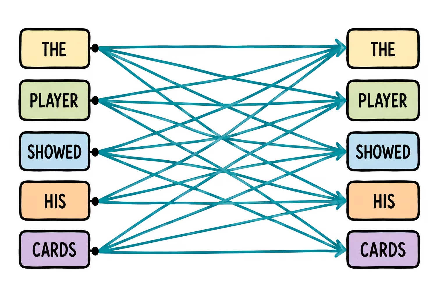
To search for these relationships, two projections are trained so that, given a sequence as input, they learn to generate two different vectors:

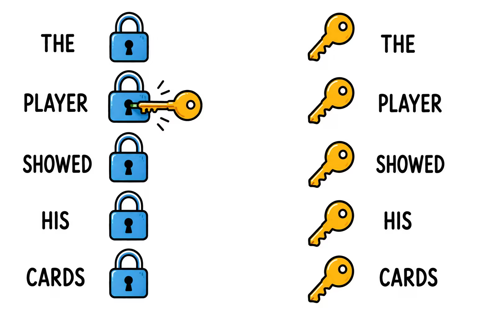
• Identifier vector 🔑 (Key): identifies the interesting properties that characterize each word.
• Search vector 🔒 (Query): describes the interesting properties that each word is looking for.

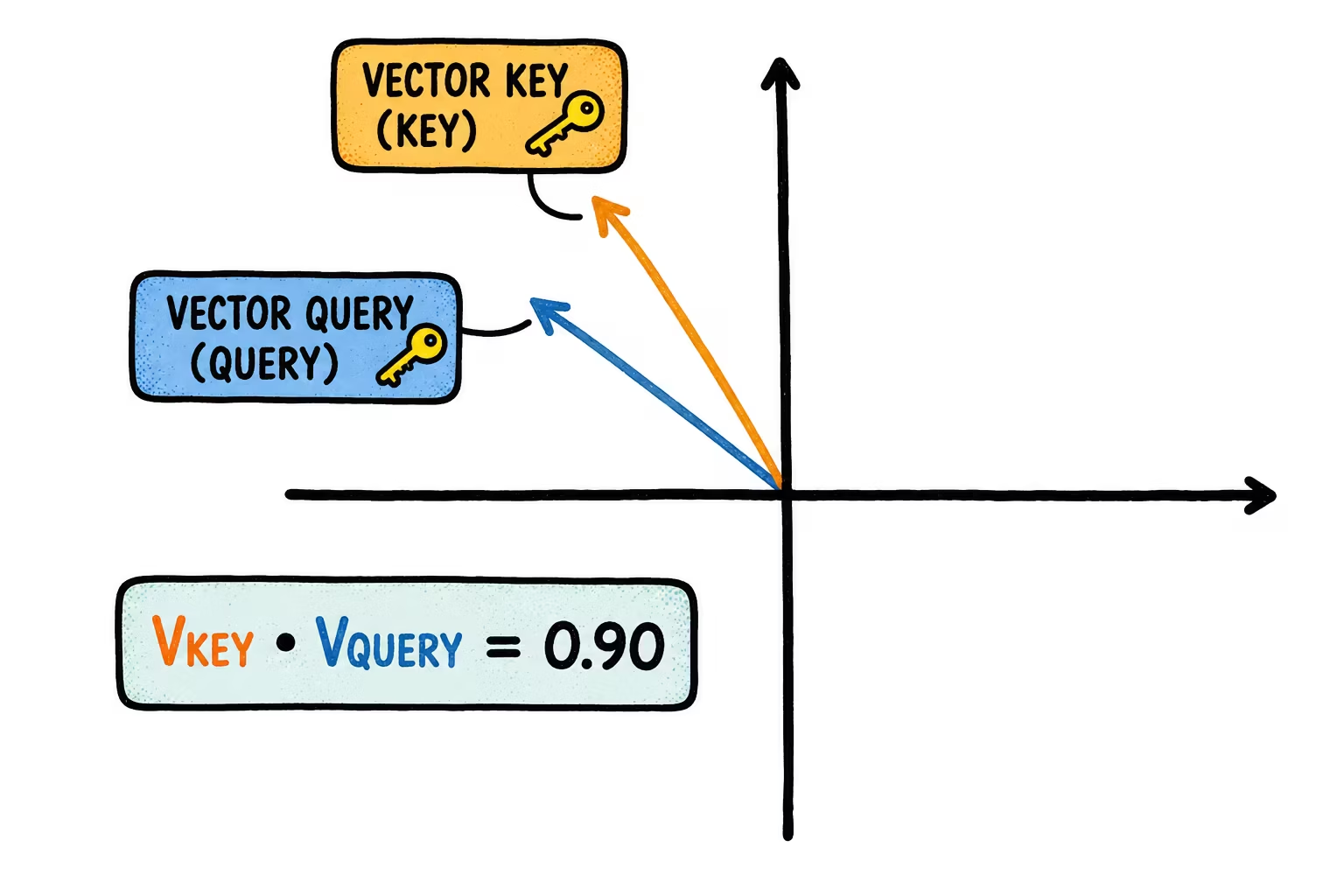
If there is some query word whose description is compatible with what the key word is looking for, a match should be generated. It's something equivalent to trying keys (identifier/key) in different locks (search/query), where the keys work with lesser or greater success.

To quantify compatibility, the dot product between the key and query vectors is used, $QK^\top$. It will be larger the more the directions of the vectors coincide (if they coincide to a large degree, that value will be high).

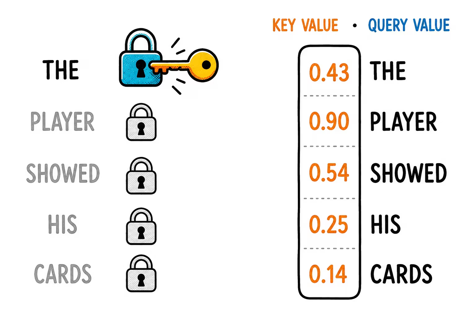
When working with high-dimensional vectors $d_k$, the sum of many products tends to produce extremely large scalar values. To smooth this out, it is divided by $\sqrt{d_k}$, normalizing the variance of the scores.

$$S=\frac{QK^\top}{\sqrt{d_k}}\qquad$$

We know this as the compatibility matrix or scores. Then, the $\operatorname{softmax}$ function is applied along each row of S to transform the scores into a probability distribution (values between 0 and 1 that add up to 1).

$$A=\operatorname{softmax}(S),\qquad$$

This is the attention vector. If a word's key fits the lock perfectly, it will get a weight close to 1 (almost total attention); if not, its weight will fall toward 0.

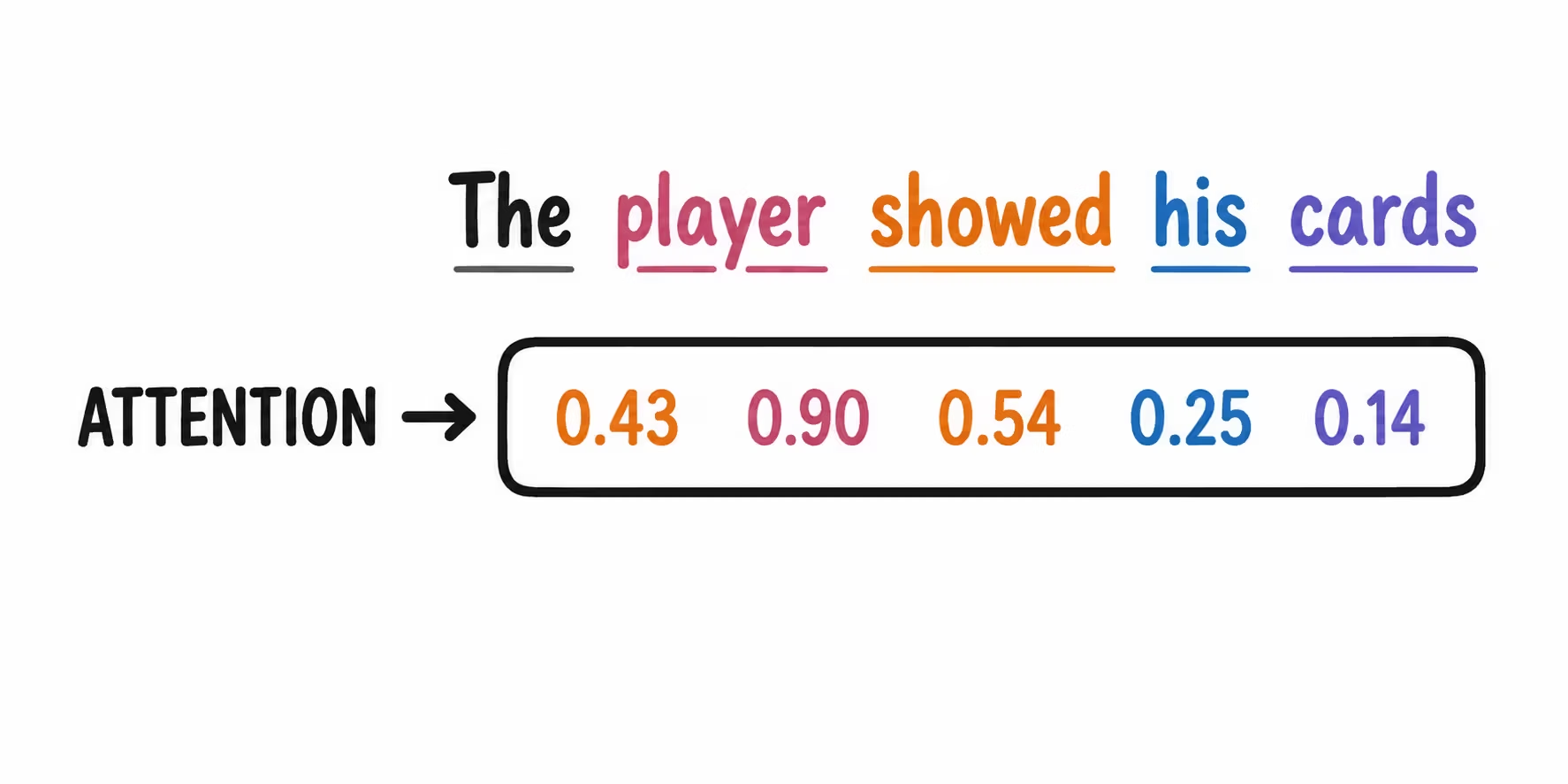
This way, unlike recurrent networks, words can be associated regardless of how far apart they are in the sentence.

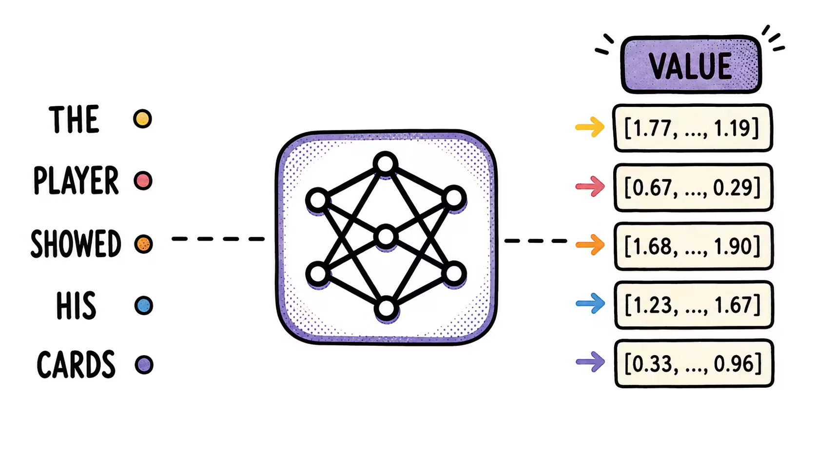
Then, there is another projection that processes each of the tokens, generating a vector known as the value vector (Value).

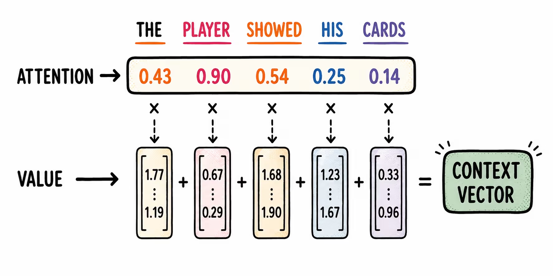
If we compute the weighted sum of the product of the attention vector with the value vector, the result is a vector that captures the context of the sentence:

$$\operatorname{Attention}(Q,K,V)=AV$$

Transformers

We had seen that with recurrent networks we mainly had two problems arising from sequential processing:

• handling very distant dependencies (long texts) is limited
• parallel training becomes impossible

Attention mechanisms partly mitigate the first problem, but the second one remains.

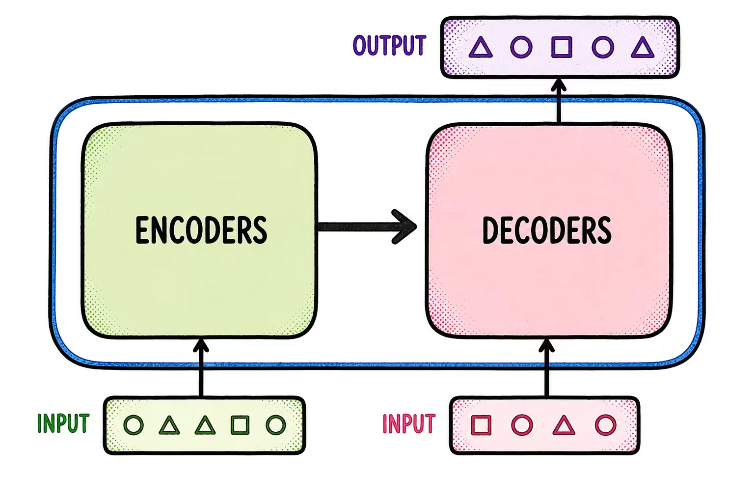
The inputs/outputs depend on the goal to be solved. Examples:

• Translation. Encoder input: sentence in language 1; decoder input: sentence in language 2; output: sentence in language 2 shifted by one unit.
• Text prediction. Encoder input: there is no encoder. Decoder input: sentence; output: next token/word.
• Time series prediction. Encoder input: time series (e.g.: T1, T2, T3, T4). Decoder input: continuation of the series (T4, T5); output: continuation of the series shifted by one unit (T5, T6).

Positional encoding

If everything is now processed at the same time, how do we know the order of the sequences?

1st approach: one option would be to add to each embedding vector another vector whose components all mark the position it occupies (absolute positioning).

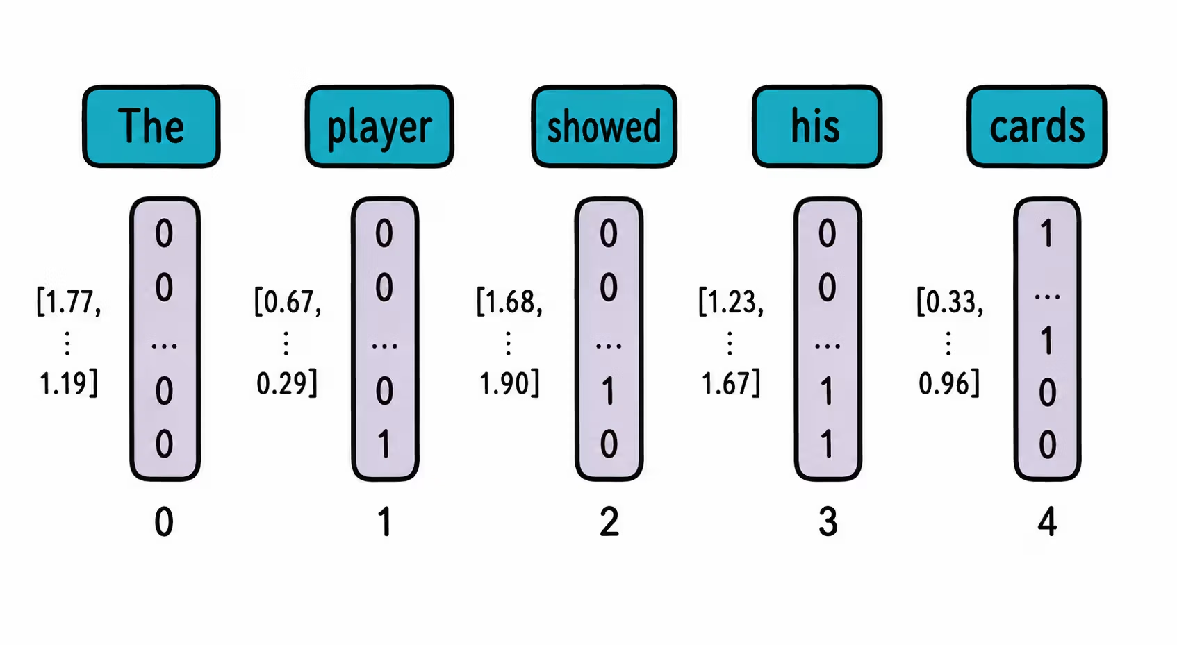
❗ Problem: if we have very long sequences, we would be adding a very large value to the last vector.

2nd approach: a solution to the previous problem would be to divide each positional vector by the number of words in the sentence, that is, to normalize the vectors.

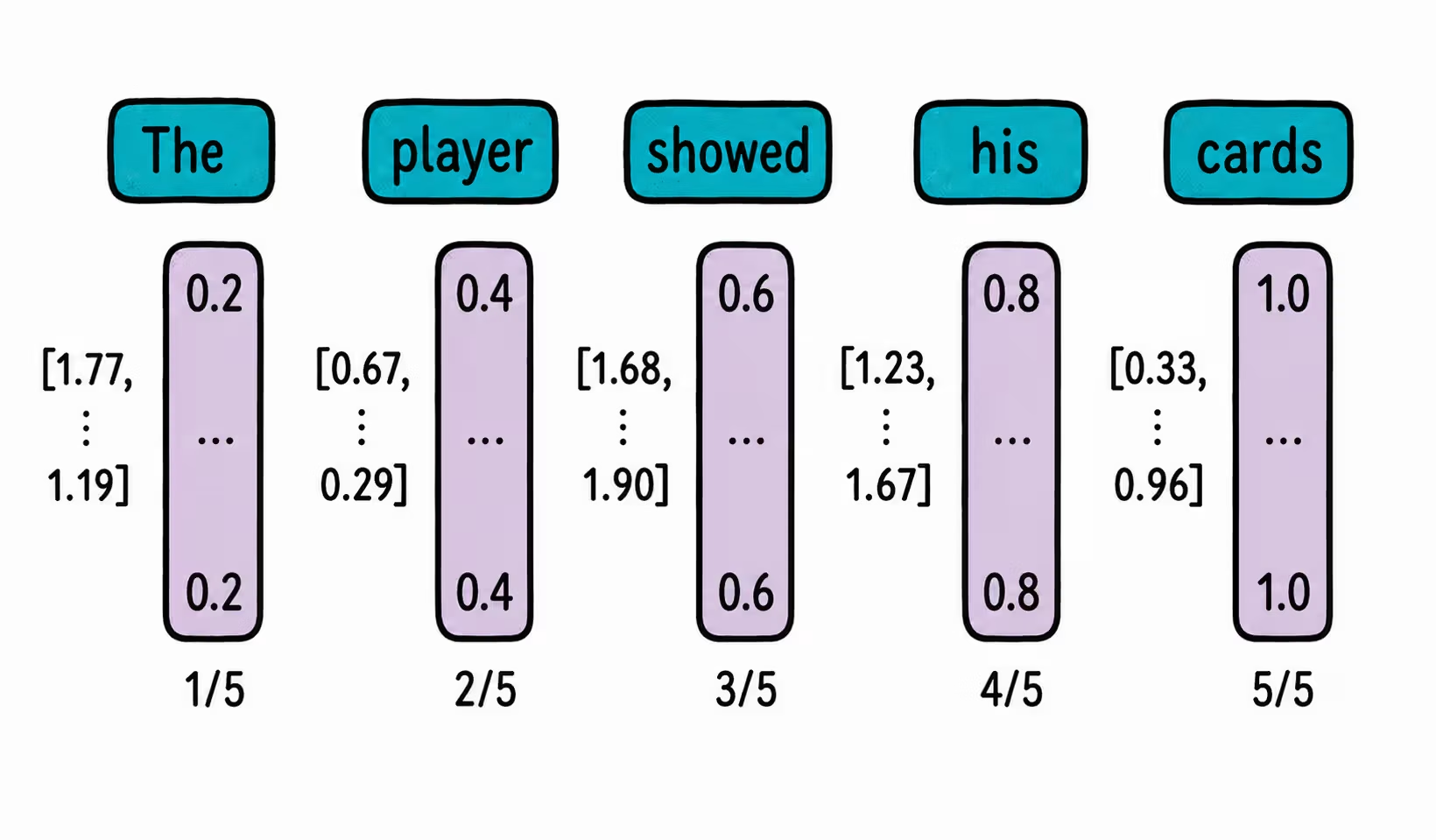
❗ Problem: what would happen if we have sequences of different lengths?

3rd approach: work only with 1s and 0s → binary encoding.

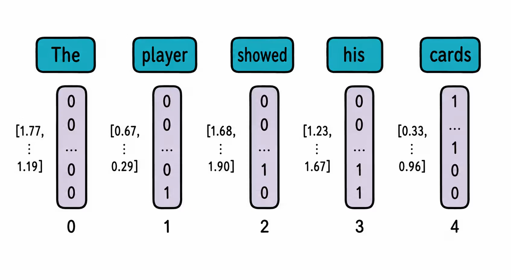
This strategy is closer to the continuous nature of neural networks. In fact, these state changes can be represented as waves oscillating at different frequencies:

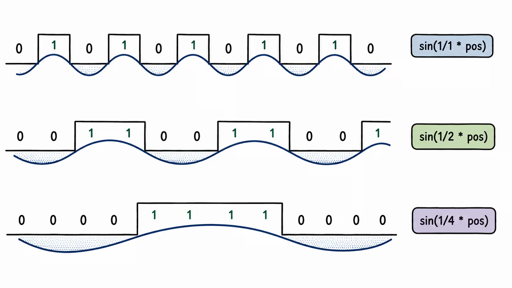
Therefore, positional encoding can be computed with a single sinusoidal function. The formula from the original paper is a bit more complex, but the intuition behind it is exactly the same:

$$PE_{(pos,\,2i)} = \sin\left(\frac{pos}{10000^{2i/d_{model}}}\right)$$ $$PE_{(pos,\,2i+1)} = \cos\left(\frac{pos}{10000^{2i/d_{model}}}\right)$$

This way, the Transformer can understand the order of the sequences passed as input (while still processing everything in parallel).

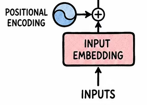
Summary

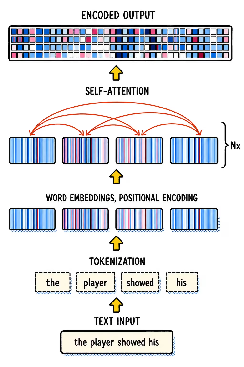
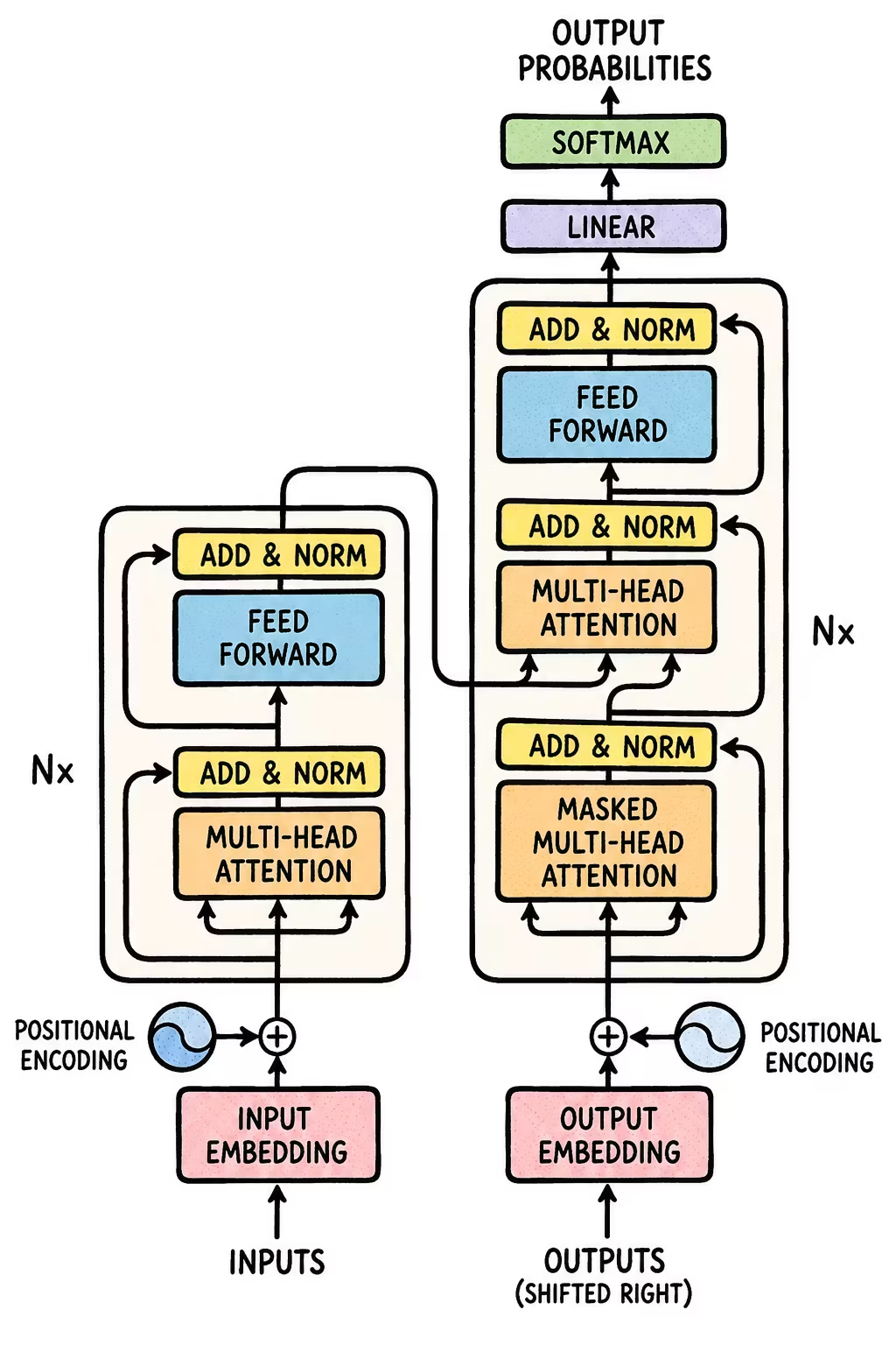
With this we already have a notion of the main components of the Transformer.

Learnable Positional Embeddings

In models such as BERT or GPT-2, the sinusoidal functions were replaced with learnable positional embeddings. That is, each position has an embedding that, instead of being deterministic, is trained, just like the word embeddings.

• Advantage: the model learns the best positional representation for its task.
• Disadvantage: it loses generalization to sequences longer than those seen during training.

RoPE (Rotary Positional Embedding)

Both sinusoidal encoding and learnable positional embeddings share the same strategy: they compute a position vector and add it to the word embedding before the sequence enters the Transformer. However, attention isn't interested in the absolute position of each word, but in the relative distance between the word asking (query) and the word being attended to (key). Adding a fixed position vector forces the model to infer that distance indirectly, by comparing two absolute positions.

RoPE^{[su2021roformer]} is a strategy adopted by more recent models, in which, instead of adding the position, it encodes it as a rotation that is applied directly to the query and key vectors within each attention layer → never to the input embedding, and never to the value vector.

The geometric idea

Rotating a 2D vector by an angle $\theta$ around the origin doesn't change its length, only its orientation. RoPE takes advantage of exactly this property: it takes the query (or key) vector of a word at position $m$, splits it into pairs of components $(x_{2i}, x_{2i+1})$, and rotates each pair by an angle proportional to $m$:

$$\begin{pmatrix} x'_{2i} \\ x'_{2i+1} \end{pmatrix} = \begin{pmatrix} \cos(m\theta_i) & -\sin(m\theta_i) \\ \sin(m\theta_i) & \cos(m\theta_i) \end{pmatrix} \begin{pmatrix} x_{2i} \\ x_{2i+1} \end{pmatrix}$$

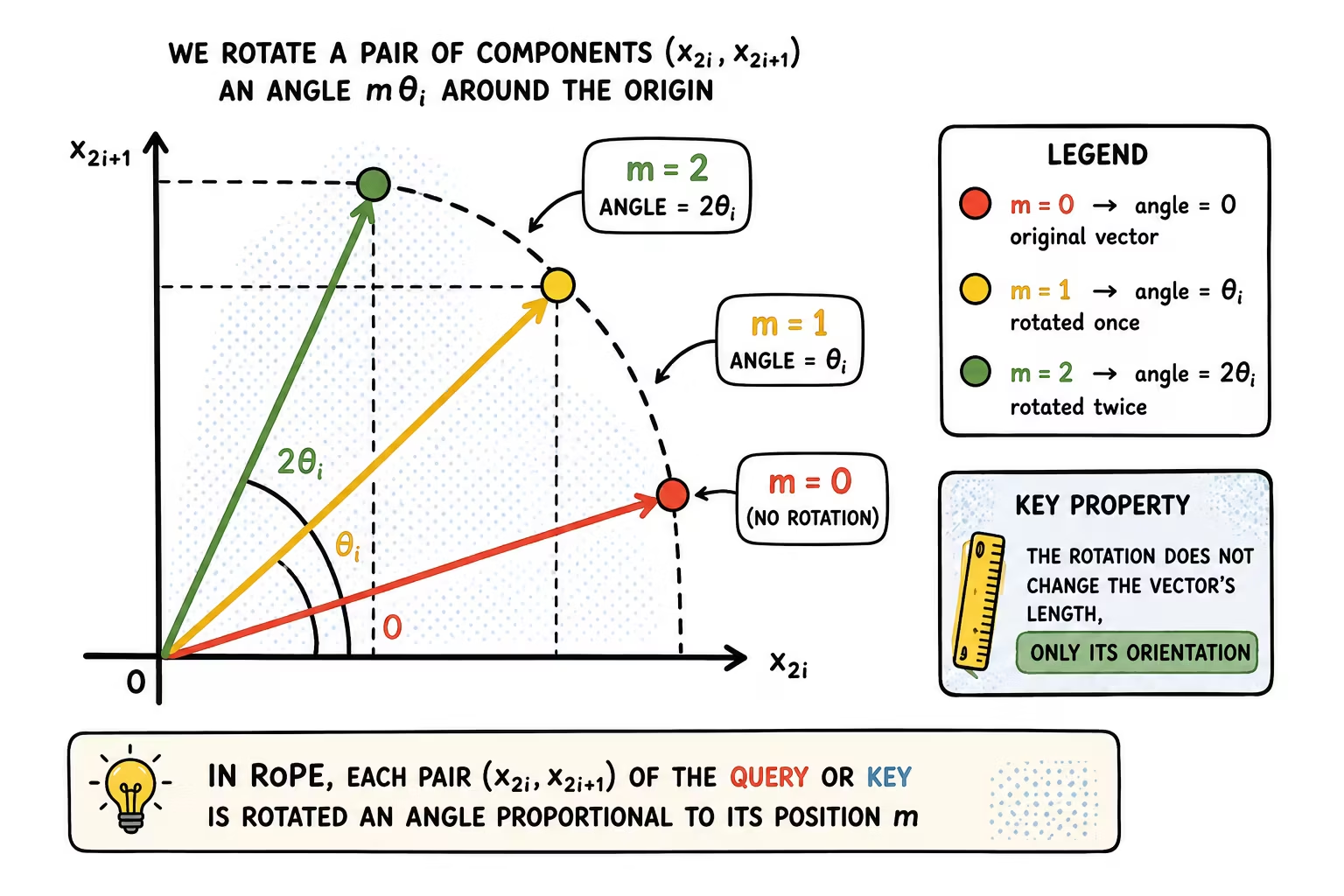
Each pair of dimensions $i$ rotates at a different frequency, $\theta_i = 10000^{-2i/d_{model}}$ → the same frequencies used by sinusoidal encoding. The first pairs (high frequency) rotate quickly and distinguish nearby positions; the last ones (low frequency) rotate slowly and capture long-range relationships. A vector of $d_{model}$ dimensions is thus treated as $d_{model}/2$ independent pairs, each rotating in its own 2D plane at its own speed. This process is applied equally to the query vector (with its position $m$) and to the key vector (with its position $n$) of each token.

Why this encodes relative position

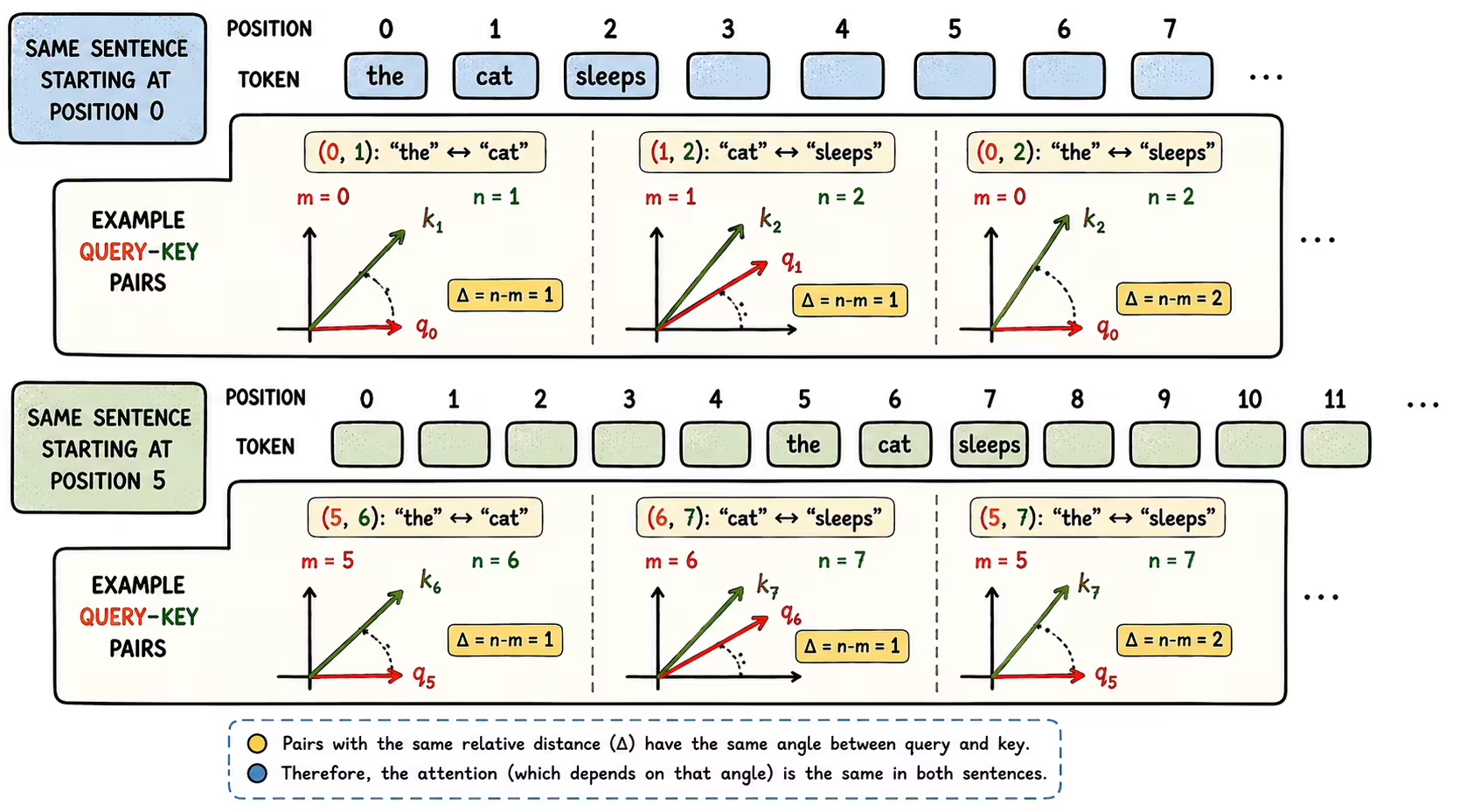
This is RoPE's key result. When computing attention, what matters is the dot product between the rotated query at position $m$ and the rotated key at position $n$. Calling $R_m$ the rotation matrix at position $m$, and taking advantage of the fact that rotations are orthogonal ($R_m^\top = R_{-m}$):

$$(R_m q)^\top (R_n k) = q^\top R_m^\top R_n k = q^\top R_{n-m} \, k$$

The result doesn't depend on $m$ and $n$ separately, but only on their difference $n-m$: the relative distance between the two words. The absolute position disappears from the equation and only the relationship between positions survives, which is exactly what attention needs to know.

Advantages over the previous approaches

• Encodes relative relationships natively, without adding anything to the embedding or learning a position table.
• Preserves the norm of the vectors: a rotation doesn't change the length of the vector, so it doesn't distort the scale of the dot products the way adding a large position vector would.
• Generalizes better to longer sequences than those seen in training, because the mechanism isn't tied to a fixed range of learned positions (although extending the context far beyond training still requires additional adjustments, such as rescaling the frequencies — techniques like NTK-aware scaling or YaRN).
• Adds no parameters: unlike learnable positional embeddings, the rotations are computed with a fixed formula, not trained.

In summary, the flow that $Q$ and $K$ follow right before computing attention becomes: embedding → linear projection to Q/K/V → rotate Q and K according to their position → dot product.

Learning process

The original Transformer combines an encoder with an autoregressive decoder. In generation tasks, that decoder is trained to predict the next token of a sequence from the previous tokens.

The decoder is given the target sequence itself as input, and that same sequence shifted by one position as output. This is what's known as teacher forcing: during training, at position $t$ the model receives the real tokens $x_1, \dots, x_t$ as input (not the ones it would generate itself) and has to predict the token $x_{t+1}$.

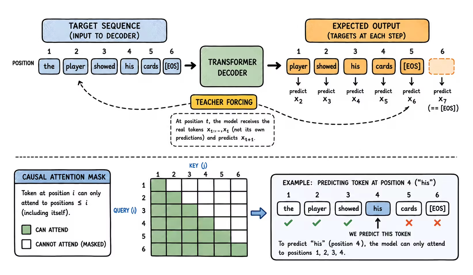
For this to work, two ingredients are needed:

• Causal mask: the decoder's self-attention is masked so that the prediction of token $t+1$ cannot "cheat" by looking at future tokens → each position can only attend to itself and the previous ones.
• Loss function: at each position, the predicted probability distribution over the vocabulary (the output of a final softmax layer) is compared with the real token using cross-entropy, and averaged across the whole sequence.

Thanks to the combination of teacher forcing and the causal mask, all positions of the sequence can be trained at once in a single forward pass → there is no need to wait for the model to predict token $t$ in order to process $t+1$.

This same idea, training by predicting the next token from the previous context, is the one that, scaled up to massive amounts of unlabeled text, becomes the pretraining paradigm of foundational language models → we'll see it in detail in the next chapter.

Extra: Vision Transformers

In ViTs ^{[dosovitskiy2020image]}, images are split into multiple sub-images (patches) that are passed to the Transformer encoder as if they were a sequence.

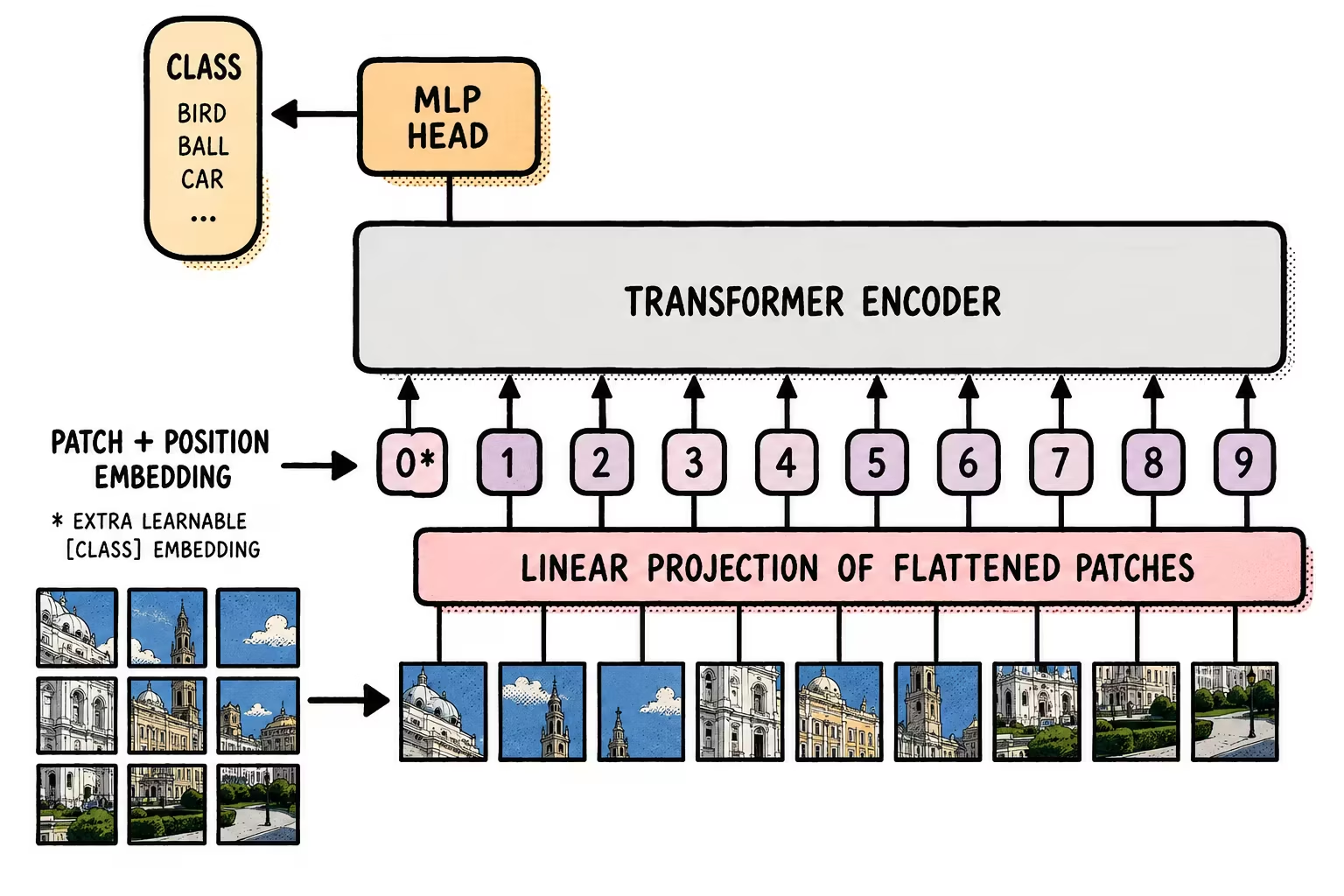
Again, since this is a Transformer that processes everything in parallel and therefore doesn't know the order of the data, it's necessary to provide it with that information.

Unlike text, where the order is sequential, in images the order between pixels matters, but it isn't strictly sequential between patches. For this reason, applying the original positional encoding doesn't make much sense. ViTs apply learnable Positional Embeddings to let the network learn the most suitable positional encoding.

That is, it's given the image and its position:

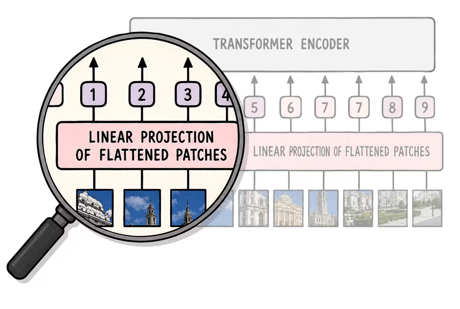
It isn't given the numbers 1, 2, 3… but rather each number is associated with a vector. These vectors are parameters that the model learns during training → learnable embeddings.

In this case, only the encoder can be trained with one of the learning paradigms we'll see in the next chapter. Once the model is pretrained, simple classifiers can be built on top of the representations obtained.

The context window

Both text and visual patches ultimately form sequences that the Transformer has to process. Those sequences cannot grow indefinitely. Each model has a context window: the maximum number of tokens it can keep available within a single inference.

When a conversation exceeds that limit, the application has to trim, summarize, or compress part of its history. The model can no longer attend directly to the original content that has fallen outside the window, even if the interface still displays the entire conversation.

To learn more